NU-WRF Version 11.5 User’s Guide

National Aeronautics and Space Administration

Goddard Space Flight Center

Greenbelt, Maryland 20771

30 Sep 2024

Introduction

This Document

This is the NASA Unified-Weather Research and Forecasting (NU-WRF) Version 11.5 User’s Guide. This document provides an overview of NU-WRF; describes how to download, compile, and run the NU-WRF software; and guides porting the software to new platforms.

This document consists of six sections and three appendices:

Introduction is the present introductory section.
NU-WRF System provides general information about the NU-WRF project and its components.
Obtaining Software provides information on obtaining a software usage agreement and the NU-WRF source code.
Building Software describes how to compile the NU-WRF software;
Front-End Workflows describes several front-end workflows that can be employed with the NU-WRF modeling system, ranging from basic weather simulation to advanced aerosol-microphysics-radiation coupling to alternate initialization methods. This includes information on new pre-processors and NASA changes to the community WRF model.
Post-Processors describes several post-processors for visualization and/or verification.
Finally, the FAQ section answers Frequently Asked Questions about NU-WRF, Porting provides guidance on porting NU-WRF to new platforms and Revisions lists the NU-WRF revision history.

Acknowledgments

The development of NU-WRF has been funded by the NASA Modeling, Analysis, and Prediction Program. The Goddard microphysics, radiation, aerosol coupling modules, and G-SDSU are developed and maintained by the Mesoscale Atmospheric Processes Laboratory at NASA Goddard Space Flight Center (GSFC). The GOCART and NASA dust aerosol emission modules are developed and maintained by the GSFC Atmospheric Chemistry and Dynamics Laboratory. The LIS, LDT, and LVT components are developed and maintained by the GSFC Hydrological Sciences Laboratory. The CASA2WRF, GEOS2WRF, GOCART2WRF, LISWRFDOMAIN, LIS4SCM, NEVS, NDVIBARENESS4WRF, and SST2WRF components are maintained by the GSFC Computational and Information Sciences and Technology Office. SST2WRF includes binary reader source code developed by Remote Sensing Systems.

Past and present contributors affiliated with the NU-WRF effort include: Kristi Arsenault, Clay Blankenship, Scott Braun, Rob Burns, Jon Case, Mian Chin, Tom Clune, David Considine, Carlos Cruz, John David, Craig Ferguson, Jim Geiger, Mei Han, Ken Harrison, Arthur Hou, Takamichi Iguchi, Jossy Jacob, Randy Kawa, Eric Kemp, Dongchul Kim, Kyu-Myong Kim, Jules Kouatchou, Anil Kumar, Sujay Kumar, William Lau, Tricia Lawston, David Liu, Yuqiong Liu, Toshi Matsui, Hamid Oloso, Christa Peters-Lidard, Chris Redder, Scott Rheingrover, Joe Santanello, Roger Shi, David Starr, Rahman Syed, Qian Tan, Wei-Kuo Tao, Zhining Tao, Eduardo Valente, Bruce Van Aartsen, Gary Wojcik, Di Wu, Jinwoong Yoo, Benjamin Zaitchik, Brad Zavodsky, Sara Zhang, Shujia Zhou, and Milija Zupanski.

The upstream community WRF, WPS, and ARWPOST components are developed and supported by the National Center for Atmospheric Research (NCAR), which is operated by the University Corporation for Atmospheric Research and sponsored by the National Science Foundation (NSF). The Kinetic Pre-Processor included with WRF-Chem was primarily developed by Dr. Adrian Sandu of the Virginia Polytechnic Institute and State University. The community RIP4 is maintained by NCAR and was developed primarily by Dr. Mark Stoelinga, formerly of the University of Washington. The UPP is developed by the National Centers for Environmental Prediction; the community version is maintained by the Developmental Testbed Center (DTC), which is sponsored by the National Oceanic and Atmospheric Administration, the United States Air Force, and the NSF. DTC also develops and maintains the community MET package. The Community PREP_CHEM_SOURCES is primarily developed by the Centro de Previsão de Tempo e Estudos Climáticos, part of the Instituto Nacional de Pesquisas Espaciais, Brazil.

NU-WRF Version 11.5, “Ekman”, is named after Vagn Walfrid Ekman, a Swedish oceanographer best known for his studies of the dynamics of ocean currents. Common oceanographic terms such as Ekman layer, Ekman spiral, and Ekman transport derive from his research.

NU-WRF System

NU-WRF has been developed at Goddard Space Flight Center (GSFC) as an observation-driven integrated modeling system representing aerosol, cloud, precipitation, and land processes at satellite-resolved scales (Peters-Lidard et al. 2015). NU-WRF is intended as a superset of the standard NCAR Advanced Research WRF [WRF-ARW; (Skamarock et al. 2008)] and incorporates:

The GSFC Land Information System [LIS; see (Kumar et al. 2006) and (Peters-Lidard et al. 2007)], coupled to WRF and also available as a stand-alone executable;
The WRF-Chem enabled version of the Goddard Chemistry Aerosols Radiation Transport model [GOCART; (Chin et al. 2002)];
GSFC radiation and microphysics schemes including revised couplings to the aerosols [(Shi et al. 2014); (Lang et al. 2014)]; and

In addition, multiple pre- and post-processors from the community and from GSFC have been collected with WRF and LIS. Taken together, the NU-WRF modeling system provides a framework for simulating aerosol and land use effects on such phenomena as floods, tropical cyclones, mesoscale convective systems, droughts, and monsoons (Peters-Lidard et al. 2015). Support also exists for treating CO $_{2}$ as a tracer, with plans to further refine into source components (anthropogenic versus biogenic). Finally, the software has been modified to use netCDF4 (http://www.unidata.ucar.edu/software/netcdf/) with HDF5 compression (https://www.hdfgroup.org/HDF5/), reducing netCDF file sizes by up to 50%.

Recently NU-WRF was incorporated into a separate, Maximum Likelihood Ensemble Filter-based atmospheric data assimilation system (NASA 2016), with the capability of assimilating cloud and precipitation-affected radiances (Zhang et al. 2015). In addition, some secondary, rarely used elements of the community WRF modeling system that are not yet included with NU-WRF may be added in the future.

Components

The NU-WRF package contains the following components and utilities:

The WRF/ component contains a modified copy of the core WRF version 4.4 modeling system [see Chapter 5 of (NCAR 2022)], the WRF-Fire wildfire library [see Appendix A of (NCAR 2022)], the WRF-Chem atmospheric chemistry library [see (Peckham et al. 2022) and (Peckham et al. 2015)], and several preprocessors (REAL, CONVERT_EMISS, TC, and NDOWN). In particular, WRF has been modified to include:
- couplings between these schemes and GOCART
- new dust emission options
- a new CO $_{2}$ tracer parameterization,
- the 2017 Goddard radiation package
This latter package was officially integrated into WRF in v4.2. WRF/ also includes LIS/LDT/LVT (in LISF/) with code modifications to both LIS and WRF-ARW to facilitate on-line coupling between the atmosphere and Noah land surface models, as well as land data assimilation (NASA 2022b).
The WPS/ component contains a modified copy of the WRF Preprocessing System version 4.4 [see Chapter 3 of (NCAR 2022)]. This includes the GEOGRID, UNGRIB, and METGRID programs used to set up a WRF domain, to interpolate static and climatological terrestrial data, to extract fields from GRIB and GRIB2 files, and to horizontally interpolate the fields to the WRF grid. This also includes the optional AVG_TSFC preprocessor, which calculates time-average surface temperatures for use in initializing small in-land lake temperatures.
The LISF/ldt/ component contains version 7.4 of the NASA Land Data Toolkit (LDT) software (NASA 2022a). This acts both as a preprocessor for LIS (including interpolation of terrestrial data to the LIS grid and separate preprocessing for data assimilation) and a postprocessor for LIS (merging dynamic fields from a LIS off-line “spin-up” simulation with static data for eventual input to WRF in LIS coupled mode).
The LISF/lvt/ component contains version 7.4 of the NASA Land Verification Toolkit (NASA 2022c) for verifying LIS land and near-surface fields against observations and gridded analyses.
The RIP4/ component contains a modified copy of the NCAR Graphics-based Read/Interpolate/Plot (Stoelinga 2006) graphical postprocessing software, version 4.6.7. Modifications include support for UMD land use data (from LIS) and WRF-Chem output.
The ARWpost/ component contains version 3.1 of the GrADS-compatible ARWpost program for visualization of output [see Chapter 9 of (NCAR 2022)].
The UPP/ component contains a modified copy of the NCEP Unified Post Processor version 3.1.1. This software can derive fields from WRF netCDF output and write in GRIB format (see (DTC 2015)).
The MET/ component contains version 10.0.0 of the Meteorological Evaluation Tools (DTC 2021) software produced by the Developmental Testbed Center. This can be used to evaluate WRF atmospheric fields converted to GRIB via UPP against observations and gridded analyses.
The Goddard Satellite Data Simulator Unit, GSDSU/(T. Matsui et al. 2014), component contains version 4.0 of the Goddard Satellite Data Simulation Unit (Toshi Matsui and Kemp 2016), which can be used to simulate satellite imagery, radar, and lidar data for comparison against actual remote-sensing observations.
The postproc/GMP/ component contains the Goddard MicroPhysics simulator, an end-to-end microphysics development tool. It reads WRF output and conducts microphysics processes for one time step. Thus, it is a very useful tool for independent code development without running a whole NU-WRF simulation. Code can be run either in a single CPU or in parallel, and users can specify input WRF output files and subset domains.
The postproc/GRAD/ component contains the Goddard RADiation (GRAD) simulator, an end-to-end radiation development tool. It reads WRF output and conducts radiative transfer for one-time step. Like GMP, it is a very useful tool for independent code development without running a whole NU-WRF simulation and code can be run serially or in parallel.
The utils/lisWrfDomain/ utility contains the NASA LISWRFDOMAIN software for customizing LDT and LIS ASCII input files so their domain(s) (grid size, resolution, and map projection) match that of WRF. It uses output from the WPS GEOGRID program to determine the reference latitude and longitude.
The utils/geos2wrf/ utility contains version 2 of the NASA GEOS2WRF software, which extracts and/or derives atmospheric data from the Goddard Earth Observing System Model Version 5 [(Rienecker et al. 2008); http://gmao.gsfc.nasa.gov/GMAO_products] for input into WRF. It also contains MERRA2WRF, which can preprocess atmospheric fields from the Modern-Era Retrospective Analysis for Research and Applications [MERRA; (Rienecker et al. 2011)] hosted by the Goddard Earth Sciences Data Information Services Center (GES DISC; http://daac.gsfc.nasa.gov), as well as MERRA-2 reanalyses (Bosilovich et al. 2015) also hosted by GES DISC. These programs essentially take the place of UNGRIB in WPS, as UNGRIB cannot read the netCDF, HDF4, or HDFEOS formats used with GEOS-5, MERRA, and MERRA-2. This includes a python script for downloading and processing MERRA-2 files from the MERRA2 data server (only works in NCCS systems).
The utils/sst2wrf/ utility contains the NASA SST2WRF preprocessor, which reads sea surface temperature (SST) analyses produced by Remote Sensing Systems (http://www.remss.com) and converts into a format readable by the WPS program METGRID. This essentially takes the place of UNGRIB as the SST data are in a non-GRIB binary format. This includes a python script for downloading data from the RSS web page.
The utils/ndviBareness4Wrf/ utility contains the NASA NDVIBARENESS4WRF preprocessor, which reads gridded Normalized Difference Vegetation Index (NDVI) data and calculates a “surface bareness” field for use by the NU-WRF dynamic dust emissions scheme. Currently, the software reads NDVI produced from the NASA Global Inventory Modeling and Mapping Studies (GIMMS) group and by the NASA Short-term Prediction Research and Transition Center (SPoRT). Both products are based on observations from the Moderate Resolution Imaging Spectroradiometer (MODIS), which is flown on the NASA Terra and Aqua satellites. The preprocessor outputs both the NDVI and the derived bareness fields in a format readable by the WPS program METGRID.
The utils/prep_chem_sources/ utility contains a modified copy version of the community PREP_CHEM_SOURCES version 1.8.3 preprocessor. This program prepares anthropogenic, biogenic, wildfire, and volcanic emissions data for further preprocessing by the WRF-Chem preprocessor CONVERT_EMISS. The NU-WRF version of PREP_CHEM_SOURCES uses the WPS map projection software to ensure consistency in interpolation. It also adds support for GFEDv4 biomass burning emissions [see (Randerson et al. 2015)], NASA QFED wildfire emissions (Darmenov and Silva 2013), support for new 72-level GOCART background fields, improved interpolation of the GOCART background fields when the WRF grid is at a relatively finer resolution, and output of data for plotting with the NASA PLOT_CHEM program.
The utils/plot_chem/ utility stores a simple NCAR Graphics based PLOT_CHEM program for visualizing the output from PREP_CHEM_SOURCES. This program is only intended for manual review and sanity checking, not for publication quality plots.
The utils/gocart2wrf/ utility is a NASA program for reading GOCART aerosol data from an offline GOCART run (Chin et al. 2002), online GOCART with GEOS-5, MERRAero (Kishcha et al. 2014), or MERRA-2 (Bosilovich et al. 2015) files; interpolate the data to the WRF grid; and then add the data to netCDF4 initial condition and lateral boundary condition (IC/LBC) files for WRF. This includes a script for downloading and processing MERRA-2 files from the GES DISC web page.
The utils/casa2wrf/ utility contains the NASA CASA2WRF preprocessor and related software to read CO $_{2}$ emissions and concentrations from the CASA biosphere model, and interpolate and append the data to the WRF netCDF4 IC/LBC files (Tao, Jacob, and Kemp 2014).
The utils/lis4scm/ utility contains the NASA LIS4SCM preprocessor to generate horizontally homogeneous conditions in a LIS parameter file (produced by LDT), an LDT output file normally generated for the WRF REAL preprocessor, and a LIS restart file. These updated files are part of the initial conditions for NU-WRF (WRF and LIS coupled) in idealized Single Column Mode (see section 5.3).

In addition, NU-WRF includes a collection of scripts to help build, test, and port the framework. These scripts are found under the unified build system written in Python to ease the compilation of the different NU-WRF components and to automatically resolve several dependencies between the components (e.g., WPS requires WRF to be compiled first). The build system is discussed in section 4.3. Furthermore, the NU-WRF build system does not currently support compilation of the 2-D “ideal” data cases nor the 3-D WRF-Fire data case [see Chapter 4 of (NCAR 2022)].

Obtaining Software

Software Usage Agreement

The release of NU-WRF software is subject to NASA legal review and requires users to sign a Software Usage Agreement. Carlos Cruz (carlos.a.cruz@nasa.gov) and Toshi Matsui (toshihisa.matsui-1@nasa.gov) are the points of contact for discussing and processing requests for the NU-WRF software.

Note there are three broad categories for software release:

US Government – Interagency Release. A representative of a US government agency should initiate contact and provide the following information:
1. The name and division of the government agency
2. The name of the Recipient of the NU-WRF source code
3. The Recipient’s title/position
4. The Recipient’s address
5. The Recipient’s phone and FAX number
6. The Recipient’s e-mail address
US Government – Project Release under a Contract. If a group working under contract or grant for a US government agency requires the NU-WRF source code for the performance of said contract or grant, then a representative should initiate contact and provide a copy of the grant or contract cover page. Information should include the following:
1. The name and division of the government agency
2. The name of the Recipient of the NU-WRF source code
3. The Recipient’s title/position
4. The Recipient’s address
5. The Recipient’s phone and FAX number
6. The Recipient’s e-mail address
7. The contract or grant number
8. The name of the Contracting Officer
9. The Contracting Officer’s phone number
10. The Contracting Officer’s e-mail address
All Others. Those who do not fall under the above two categories but who wish to use NU-WRF software should initiate contact to discuss possibilities for collaborating. Note, however, that NASA cannot accept all requests due to legal constraints.

NUWRF Repository

Current source development is managed in a GitLab repository at (https://git.smce.nasa.gov/astg/nuwrf/nu-wrf-dev). To get access the repository contact Carlos Cruz (carlos.a.cruz@nasa.gov). Once access is granted, the user can obtain the source code using the following command [1].

git clone --recurse-submodules git@git.smce.nasa.gov:astg/nuwrf/nu-wrf-dev.git

Note that you should use the develop branch which should be not only production-ready but also will contain updates and bug fixes. Developers who wish to collaborate are encouraged to clone the Git repository and create their feature branches in their local repositories. Later, these features can be merged into the develop or master branch, via a pull request. This process requires that the code pass certain testing and validation criteria and finally be approved by the NU-WRF core developers. For more information using Git with NU-WRF see https://nuwrf.gsfc.nasa.gov/sites/default/files/docs/git-intro.pdf.

Tar File

Users can also be provided with a compressed tar file containing the entire NU-WRF source code distribution. However, it is strongly recommended that users access the source code using the Git repository. Also, note that only NU-WRF project members have access to tar files pre-staged on the NASA Discover and Pleaides supercomputers. Two variants are available: gzip compressed (nu-wrf_v11.5-wrf46-lisf.tgz) and bzip2 compressed (nu-wrf_v11.5-wrf46-lisf.tar.bz2). Bzip2 compression generates slightly smaller files but can take considerably longer to decompress.

To untar, type either:

tar -zxf nu-wrf_v11.5-wrf46-lisf.tgz

or

bunzip2 nu-wrf_v11.5-wrf46-lisf.tar.bz2

tar -xf nu-wrf_v11.5-wrf46-lisf.tar

A nuwrf_v11.5-wrf46-lisf/ directory should be created.

Directory Structure

The source code directory structure is as follows:

The GSDSU/, LISF/, utils/, WPS/, and WRF/ folders contain the source codes summarized in the Components section above.
ARWpost/, RIP4/, UPP/ and MET/ components are automatically built on the Discover system. On non-discover systems, users will be prompted to download the component(s) allowing them to be built. Copies of RIP4/ and UPP/, which contain NU-WRF specific enhancements can be provided upon request.
The docs/ folder contains reStructuredText documentation to generate this document (in docs/userguide/) as well as tutorial documentation (in docs/tutorial/).
The scripts/ folder contains various scripts for various tasks including building NU-WRF and running regression tests.
- Sample input files for RIP4 are stored in the rip/ subfolder.
- The other/ subfolder contains scripts that facilitate the installation of the required NU-WRF libraries (see External Libraries and Tools) and a script to set up the correct module environment on supported platforms.
- Finally, the python/ subfolder contains5 subfolders:
  - A utils/ subfolder with Python scripts to download SST data from NASA SPoRT, SSTRSS data from http://data.remss.com/, and MERRA data from NASA. There are also other Python utilities that can be used in specific workflows.
  - A build/ subfolder with scripts and configuration files used to build NU-WRF including.
  - A regression/ subfolder with scripts and configuration files used to regression test NU-WRF.
  - A shared/ subfolder with scripts shared by other scripts.
  - A devel/ subfolder with a script to generate a release tarball.
The testcases/ folder contains sample namelist and other input files for NU-WRF for different configurations (simple WRF, WRF with LIS, WRF-Chem, and WRF-KPP) used by the regression testing mechanism. The tutorial/ folder contains sample namelist and other input files used for the NU-WRF tutorials (https://nuwrf.gsfc.nasa.gov/nu-wrf-tutorials).

The main directory also includes a small bash script that interfaces with the NU-WRF build system (discussed in

Build System) and a README file.

Building Software

Compilers

The NU-WRF source code requires Fortran 90/2003, C, and C++ compilers. The development version supports Intel compilers. (ifort, icc, and icpc) on Discover (version 2021.4.0 ) and Pleiades (version 2020.4.304). GCC (version 12.3 on Discover, 9.3 on Pleiades) is also required for library compatibility for icpc. The master branch also works with GNU compilers and OpenMPI on Discover.

External Libraries and Tools

A large number of third-party libraries must be installed before building NU-WRF. Except as noted, the libraries must be compiled using the same compilers as NU-WRF, and it is highly recommended that static library files be created and linked rather than shared object. Included with the NU-WRF source code are scripts (see scripts/other/baselibs.*) that facilitate the installation of all software packages on Discover and Pleiades. The scripts can be adapted to other systems with modifications. The list of libraries is as follows:

An MPI library. (By default, NU-WRF uses Intel MPI on Discover and Pleiades. )
BOXMG 0.1 (Used to build with WRF_ELEC option).
BUFRLIB 11.0
CAIRO 1.14.8
ECCODES 2.23.0
ESMF 8.5.0 compiled with MPI support.
FORTRANGIS 3.0
FREETYPE 2.11.0
FLEX (can use precompiled system binary on Linux).
G2CLIB 1.6.0
GDAL 2.4.4
GEOTIFF 1.5.1
GHOSTSCRIPT 8.11
GRIB_API 1.17.0
GSL 2.3
HDF4 4.2.16
HDF5 1.14.3
HDF-EOS 2.3.0
JASPER 2.0.14
JPEG 9b.
LIBGEOTIFF 1.7.1.
LIBPNG 1.6.37.
NCAR Graphics 6.0.0. (Newer versions of NCAR Graphics require compilation and linking to the CAIRO library, which is currently only supported by MET.)
NETCDF 4.9.2 (C library), NETCDF-Fortran 4.6.1, and NETCDF-CXX 4.3.0.1 (C++ library), built with HDF5 compression.
OPENJPEG 2.5.2.
PROJ 9.3.
PIXMAN 0.40.0.
SQLITE 3.43.02
YACC (can use preinstalled version on Linux).
ZLIB 1.2.11.

In addition to the above libraries you may need to install the curl library, if not installed on your system. NU-WRF also requires perl, python3, bash, tcsh, gmake, sed, awk, m4, and the UNIX uname command to be available on the computer. The tarballs for the above packages can be obtained from: https://portal.nccs.nasa.gov/datashare/astg/nuwrf/baselibs/

Build System

Each component of the NU-WRF modeling system has a unique compilation mechanism, ranging from simple Makefiles to sophisticated Perl and shell scripts. To make it easier for the user to create desired executables and to more easily resolve dependencies between components, NU-WRF includes a build layer that glues together the entire framework. The build layer consists of a Python3-based script system configured by a config Python file, basically a text file with a particular structure readable by Python, and used to define the build environment, library paths and the build options.

The build system is shipped with the code and is found in the scripts/python/build subfolder. It includes a configuration file nu-wrf.cfg that contains settings for Discover and Pleiades but can be easily configurable for other systems. The settings in the configuration file allow users to specify configure options for the ARWPOST, RIP4, UPP, WPS, and WRF components, as well as template Makefile names for the GSDSU, LVT, and MET components. Not all components need a configuration (e.g. utils) but those that do need it are specified in separate sections. The provided configuration file should aid in porting NU-WRF to work with new compilers, MPI implementations, and/or operating systems, a process discussed more fully in the Porting NU-WRF section.

Invoking the build system is done in the top-level NU-WRF directory by executing the build.sh script. The build.sh script represents a thin layer over the Python build system. Running build.sh without arguments will print a usage page with the following information:

Target. A required argument that defines the NU-WRF component to build. See list of valid targets below.
Installation. The -p, –prefix flag followed by a path will install all built executables in the specified path. If the flag is skipped, build.sh will install the executables in the model directory.
Configuration. The -c, –config flag followed by the name of a configuration file specifying critical environment variables (e.g., the path to the netCDF library). Users may develop their own configuration file to customize settings (see Porting NU-WRF). If the config flag is skipped, build.sh will default to nu-wrf.cfg which works on Discover and Pleiades systems. The software will exit if it is on an unrecognized computer.
Options. The -o, –options flag specifies the target options. Valid options are cleanfirst, debug, rebuild, and/or nest=n where n is an integer ranging from 1 to 3. Multiple options must be comma-separated, e.g. cleanfirst,debug,nest=2. Note that only one nest option can be specified at a time.
- The cleanfirst option will cause the build system to “clean” a target (delete object files and static libraries) before starting compilation.
- The debug option forces some build subsystems (WRF, WPS, LISF, utils) to use alternative compilation flags set in the configuration file (e.g., for disabling optimization and turning on run-time array bounds checking). This option is currently ignored by other (ARWpost, GSDSU, MET, RIP4, UPP) NU-WRF components.
- The rebuild option is used to re-build the WRF executable - when only WRF code is modified - while skipping LIS re-compilation. It can thus speed up the regeneration of the WRF executable. It has no effect on other components.
- The nest=n option specifies compiling WRF with basic nesting (n=1), preset-moves nesting (n=2), or vortex-tracking nesting (n=3). Basic nesting is assumed by default. Note that WRF cannot be run coupled to LIS if preset-moves or vortex-tracking nesting is used. Similarly, WRF-Chem only runs with basic nesting.
The -e flag generates a file, nu-wrf.envs, that specifies all the NU-WRF configuration variables in a bash-script format. This can be useful for debugging or porting to other systems.
Targets. At least one target is required and multiple targets must be comma-separated. The recognized targets are (note that all* and ideal* targets are mutually exclusive):
- The all target compiles all executables without WRF-Chem.
- The allchem target compiles all executables with WRF-Chem but without the Kinetic Pre-Processor.
- The allclean target deletes all executables, object files, and static libraries.
- The allkpp target compiles all executables with WRF-Chem and including the Kinetic Pre-Processor.
- The arwpost target compiles executables in the ARWpost/ directory.
- The casa2wrf target compiles executables in the utils/casa2wrf/ directory.
- The chem target compiles executables in the WRF/ directory – except for LIS – with WRF-Chem support but without the Kinetic Pre-Processor. The compiled executables include CONVERT_EMISS.
- The gocart2wrf target compiles executables in the utils/gocart2wrf/ directory.
- The gsdsu target compiles executables in the GSDSU/ directory.
- The ideal_* targets compile ideal preprocessors in the WRF/ directory. These include:
  - ideal_scm_lis_xy: Produces inputs for running WRF-LIS in Single Column Mode.
  - ideal_b_wave Baroclinically unstable jet u(y,z) on an f-plane.
  - ideal_convrad: Idealized 3d convective-radiative equilibrium test with constant SST and full physics at cloud-resolving 1 km grid size.
  - ideal_heldsuarez: Held-Suarez coarse-resolution global forecast model.
  - ideal_les: An idealized large-eddy simulation (LES).
  - ideal_quarter_ss: 3D quarter-circle shear supercell simulation.
  - ideal_scm_xy: Single column model.
  - ideal_tropical_cyclone: Idealized tropical cyclone on an f-plane with constant SST in a specified environment.
- The kpp target compiles executables in the WRF/ directory – except for LIS – with WRF-Chem and Kinetic Pre-Processor support. The compiled executables include CONVERT_EMISS.
- The ldt target compiles executables in the LISF/ldt/ directory.
- The lis target compiles the LIS standalone executable in the LISF/lis/make/ directory.
- The lisWrfDomain target compiles executables in the utils/lisWrfDomain/ directory.
- The lis4scm target compiles executables in the utils/lis4scm directory.
- The lvt target compiles executables in the LISF/lvt/ directory.
- The geos2wrf target compiles executables in the utils/geos2wrf/ directory (both GEOS2WPS and MERRA2WRF).
- The met target compiles executables in the MET/ directory.
- The ndviBareness4Wrf target compiles executables in the
  
  utils/ndviBareness4Wrf/ directory.
- The plot_chem target compiles executables in the utils/plot_chem/ directory.
- The prep_chem_sources target compiles executables in the
  
  utils/prep_chem_sources/ directory.
- The rip target compiles executables in the RIP4/ directory.
- The sst2wrf target compiles executables in the utils/sst2wrf/ directory.
- The upp target compiles executables in the UPP/ directory.
- The utils target compiles all the executables in the utils/ directory.
- The wps target compiles executables in the WPS/ directory.
- The wrf target compiles executables in the WRF/ directory with LIS-coupling support and without WRF-Chem support.
- The wrfonly is like the wrf target but without LIS coupling support. Use this option when not using any LISF packages and thus significantly speed up compilation.

One complication addressed by the build system is that the WPS and UPP components are dependent on libraries and object files in the WRF/ directory. To account for this, the wrf target will be automatically built if necessary for WPS and/or UPP, even if the wrf target is not listed on the command line.

A second complication is that the coupling of LIS to WRF requires linking the WRF/ code to the ESMF and ZLIB libraries. As a result, the configure.wrf file [see Chapter 2 of (NCAR 2022)] is modified to link against these libraries. A similar modification occurs for UPP. (No modification is needed for WPS as long as WPS is compiled with GRIB2 support.)

Finally, if there are dependent components (WRF, WPS, UPP, LIS) that have been built with different compilation flags, compiler versions, or with/without chemistry, that will result in cleaning the associated directories.

The most straightforward way to compile the full NU-WRF system on Discover or Pleiades is to type ./build.sh all in the top-level directory. If chemistry is required, the command is ./build.sh allchem (./build.sh allkpp if KPP-enabled chemistry is needed). To fully clean the entire system, run ./build.sh allclean.

Finally, the user can selectively build components by listing specific targets. For example, to build the WRF model without chemistry along with WPS and UPP, type ./build.sh wrf,wps,upp.

LIBDIR_TAG

As discussed earlier (section External Libraries and Tools), a large number of external libraries, or baselibs, must be installed before NU-WRF can be built. More importantly, these baselibs must be compiled using the same compilers as NU-WRF. Thus, the build system parses the configuration file, nu-wrf.cfg, and, if on Discover or Pleiades systems, it uses pre-installed baselibs determined by the value of the LIBDIR_TAG environment variable set in scripts/other/set_module_env.bash. However, when porting the code to a different system and/or using a newer compiler the environment variable must be set by the user in the configuration file.

For more information see Porting NU-WRF.

Front-End Workflows

In this section we will summarize several “front-end” workflows involving the main NU-WRF model and different pre-processors. (Post-processing is discussed here). The intent is to illustrate the roles of the pre-processors within the NU-WRF system, and to show several different configurations possible with NU-WRF (e.g., advanced land surface initialization, aerosol coupling, and CO $_{2}$ tracer simulation). Finally, note that these workflows can be executed, end-to-end, as defined by regression test templates which are discussed later in this chapter.

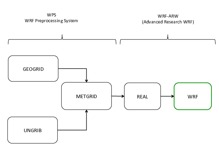
Basic Workflow

This is the simplest approach to running simulations with NU-WRF. Neither chemistry nor advanced land surface initialization are used, so the user should compile NU-WRF with ./build.sh wrf,wps.

WPS: The user must edit a namelist.wps file to customize the WRF domains, set the start and end dates, set the file formats, and provide information on desired terrestrial data and file prefixes. Sample namelist.wps files can be found in the WPS/, defaults/, and testcases/ directories. The user must then run the following programs [see Chapter 3 of NCAR 2022].
- GEOGRID. This program will interpolate static and climatological terrestrial data (land use, albedo, vegetation greenness, etc) to each WRF grid. The user should use the GEOGRID.TBL.ARW located in the WPS/geogrid/ directory to specify interpolation options for each dataset selected in namelist.wps. (Alternative GEOGRID.TBL.ARW.* files are available for chemistry cases.) The user is also responsible for obtaining the geog/ dataset from NCAR for processing by GEOGRID. Sample run scripts are available in the scripts/ directory.
- link_grib.csh. This script is used to create symbolic links to the GRIB or GRIB2 files that are to be processed. The links follow a particular naming convention (GRIBFILE.AAA, GRIBFILE.AAB, …, GRIBFILE.ZZZ) that is required by UNGRIB.
- UNGRIB. This program will read GRIB or GRIB2 files with dynamic meteorological and dynamic terrestrial data (soil moisture, soil temperature, sea surface temperature, sea ice, etc) and write specific fields in WPS intermediate format. If necessary the user is also responsible for obtaining the GRIB/GRIB2 data and store it in an appropriate location. The user must select an appropriate Vtable file in WPS/ungrib/Variable_Tables/ to specify the fields to be extracted.
- METGRID. This program will horizontally interpolate the output from UNGRIB to the WRF domains, and combine them with the output from GEOGRID. The user must select the METGRID.TBL.ARW file to specify the interpolation methods used by METGRID for each field.
REAL. This program will vertically interpolate the METGRID output to the WRF grid, and create initial and lateral boundary condition files. REAL is described in Chapters 4 and 5 of NCAR 2022. The user must edit a namelist.input file to specify the WRF domains, start and end times, and WRF physics configurations for REAL. A standard WRF land surface model should be selected for this workflow. No chemistry options can be selected. Sample namelist.input files are available in the testcases/ directory.
WRF. This program will perform a numerical weather prediction simulation using the data from REAL. The user needs to change the namelist.input file for specific run cases. A sample namelist.input file can be found in the WRF/run/ directory and in testcases/. WRF is described in Chapter 5 of NCAR 2022. In addition to the normal WRF physics options, the user can specify the new Goddard microphysics (mp_physics=7), and the Goddard 2017 radiation scheme (ra_lw_physics=5 for longwave, and ra_sw_physics=5 for shortwave respectively), all without aerosol coupling. The 2017 radiation scheme requires users to create a symbolic link to one file, WRF/run/BROADBAND_CLOUD_GODDARD.bin, and to put that link in the directory where the model is run.

A feature added to NU-WRF is the calculation of mean integrated vapor transport. The user may adjust the time-averaging period for this diagnostic by changing the IVT_INTERVAL flag in the &time_control block of namelist.input. A value of 0 indicates instantaneous values will be output as the “means”, while positive values indicate averaging time periods in minutes.

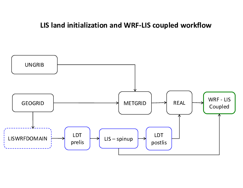
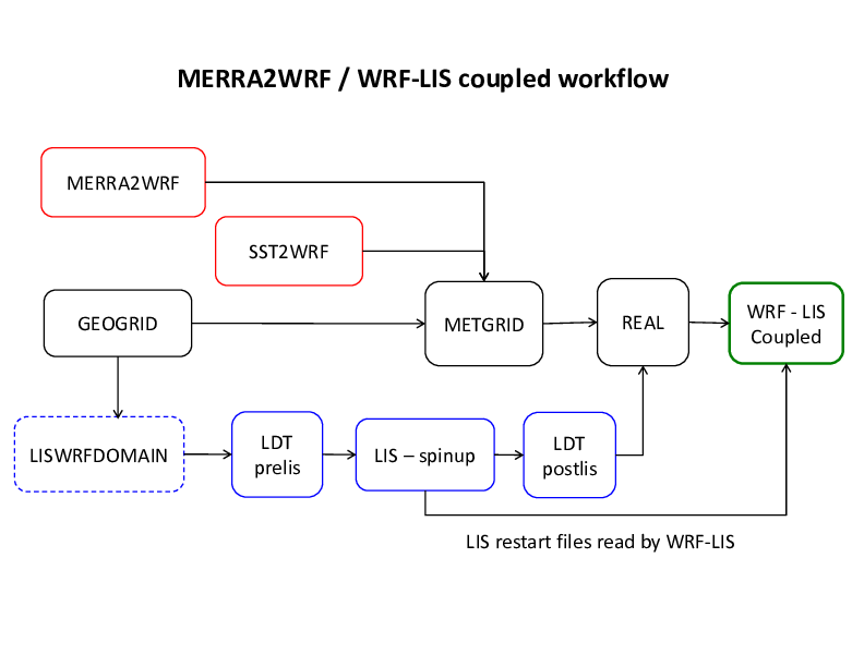
Land Surface Initialization and LIS Coupling

This is a more advanced approach to running simulations with NU-WRF. Instead of using land surface fields interpolated from a coarser model or reanalysis, a custom-made land surface state is created by LIS on the same grid and with the same terrestrial data and land surface physics as WRF. WRF will then call LIS on each advective time step, providing atmospheric forcing data and receiving land surface data (fluxes, albedo, etc) in return.

For simplicity, this workflow uses no chemistry, so the user should compile NU-WRF with ./build.sh wrf,wps,lis,ldt,lisWrfDomain. However, an advanced user can combine this workflow with one of the chemistry workflows described further down; in that case, the user should replace the wrf target with chem (or with kpp if using KPP-based chemistry).

WPS. These steps are identical to those WPS steps in the Basic Workflow section above.
LISWRFDOMAIN. The user must provide a ldt.config file (used by LDT) and a lis.config file (used by LIS). The LISWRFDOMAIN software will read the namelist.wps file and the netCDF4 output files from GEOGRID, and copy the WRF grid information to the two configuration files. LISWRFDOMAIN is divided into two executables: lisWrfDomain (a Fortran compiled program found in utils/bin/) and lisWrfDomain.py (a Python wrapper script found in scripts/python/utils/).

The software can be run as ./lisWrfDomain.py DOMAINPROG LISCONFIG LDTCONFIG WPSDIR, where DOMAINPROG is the path to lisWrfDomain, LISCONFIG is the path to lis.config, LDTCONFIG is the path to ldt.config, and WPSDIR is the directory containing namelist.wps and the GEOGRID netCDF4 output files.

Sample configuration files are provided in the testcases/ directory.
LDT. The user must further customize the ldt.config file and a separate parameter attributes file to specify the static and climatological terrestrial data to be processed in “LSM parameter processing mode” [see NASA 2022a]. The following settings are recommended/supported (please refer to the LDT documentation):
- NoahMP.3.6 is the recommended land surface model;
- MODIS is the recommended land use dataset (UMD and USGS are also supported);
- SRTM30 is the recommended terrain elevation dataset (GTOPO30 is also supported);
- STATSGOFAO is the recommended soil texture dataset;
- NCEP monthly climatological albedo and and max snow free albedo are recommended;
- NCEP monthly climatological and maximum/minimum vegetation greenness are recommended;
- NCEP slope type is recommended;
- Use of the “slope-aspect correction” is recommended to improve soil moisture spin-ups; and
- ISLSCP1 deep soil temperature with terrain lapse-rate correction is recommended (not using the lapse rate correction could result in warm biases in high terrain).
LIS. The user must further customize lis.config for a “retrospective” run. This includes specifying the start and end dates of the “spin-up” simulation, identifying the LDT datasets, specifying the land surface model, and identifying the atmospheric forcing datasets. The user must also customize a forcing variables list file compatible with the forcing dataset, and a model output attributes file. All these files are described in more detail in NASA 2022b. Sample forcing variable and output attribute files are provided in the testcases/ directory.
LDT. After running LIS, it is necessary to rerun LDT in “NUWRF preprocessing for real” mode. This requires modifications to ldt.config to specify the static output file from LDT and the dynamic output file from LIS. Fields from both will be combined and written to a new netCDF output file for use by REAL. Sample files are given in testcases/.
REAL. REAL is run similarly to the Basic Workflow configuration, except that it also reads the static and dynamic land surface data collected by LDT. For this to work, the namelist.input file must include an additional namelist block:
```
 &lis
   lis_landcover_type = 2,
   lis_filename = "lis4real_input.d01.nc"
   use_lis_noahmp = "yes"
/
```
Here lis_landcover_type specifies the land use system used with LIS and LDT (1 = USGS, 2 = MODIS, 3 = UMD); lis_filename is an array of character strings specifying the combined LDT/LIS files for each WRF domain; use_lis_noahmp specifies that a NOAHMP LSM will be used, otherwise (“no“ option) a regular Noah LSM is assumed; use_lis_urban specifies that urban physics values generated by the LIS framework will be updated (coupled) into the WRF surface driver.

In addition, the user must specify LIS as the land surface model selection with WRF (sf_surface_physics=55).

The resulting initial and lateral boundary conditions will replace the land surface fields from UNGRIB with those from LDT/LIS.
WRF with LIS. Running WRF in this case is similar to the Basic Workflow case, except that WRF will also read the lis.config file and the LIS restart files that were produced during the “retrospective” run. The user must modify lis.config to run in “WRF coupling mode”, and specify forcing_variables_wrfcplmode.txt as the forcing variables list file. The start mode must also be changed to “restart”, and the time step for each LIS domain must match that used with WRF (specified in namelist.input).

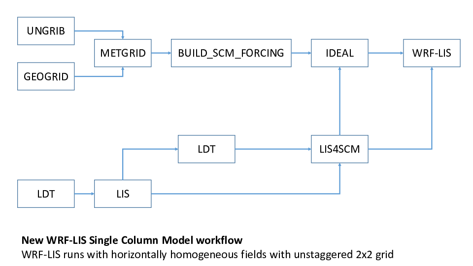
Single Column Model with LIS Coupling

Recently, an idealized configuration for WRF with LIS coupling was added to NU-WRF: the WRF-LIS Single Column Model (SCM) mode. Based on the community SCM mode, the WRF-LIS SCM configuration runs with a $3 \times 3$ staggered horizontal grid ( $2 \times 2$ for the unstaggered mass grid) and horizontally homogeneous initial conditions. Boundary conditions are periodic. To run the WRF-LIS SCM, the system must be compiled using ./build.sh ideal_scm_lis_xy,wps,lis,ldt,lis4scm, followed by this workflow:

GEOGRID. Run GEOGRID in a $3 \times 3$ staggered grid centered on a point of interest. Any normal map projection can be used (i.e., Lambert Conformal, Mercator, or Polar Stereographic), but the spatial grid resolution should be small ( $\sim 1$ km) to make the projection approximately Cartesian.
UNGRIB. Run UNGRIB to extract initial conditions from a suitable external dataset.
METGRID. Run METGRID to merge the GEOGRID and UNGRIB output together.
BUILD_SCM_FORCING. Configure and run build_scm_forcing.bash in testcases/wrflis/scm. This shell script runs the build_scm_forcing.ncl script under the hood, which extracts column initial conditions and writes them in profile_init.txt and surface_init.txt. (Advanced options also exist to generate forcing data and ensemble perturbations, but these have not been tested yet.)
LDT. Run LDT in “LSM parameter processing mode”. Use a $2 \times 2$ unstaggered grid with the point of interest at the center of the southwest grid box. A latitude-longitude map projection can be used, but the grid spatial resolution should match that of GEOGRID.
LIS. Run LIS in “retrospective” mode using the same grid configuration as LDT.
LDT. Rerun LDT in “NUWRF preprocessing for real” mode.
LIS4SCM. Edit the namelist.lis4scm file in utils/lis4scm/input/ to enter (1) the name of a LIS restart file generated by the retrospective run, (2) the output file generated by LDT when preprocessing for real, and (3) the parameter file generated by LDT for LIS. Then run LIS4SCM. This program will modify the three data files and make them horizontally homogeneous by copying the values in the southwest corner to the remainder of the grid.
IDEAL. Edit a namelist.input file:
- Make sure to specify a $3 \times 3$ grid and the same spatial resolution used by GEOGRID.
- Make sure to set io_form_auxinput3 to zero in namelist block &time_control (unless using idealized forcing, which has not been tested).
- Make sure to set the &lis namelist block settings to use the output file generated by LDT for real after it has been modified by LIS4SCM.
- Make sure to set the &scm namelist block [see Chapter 5 of NCAR 2022]. Note that the settings for land use, soil type, vegetation fraction, and canopy water are ignored, as these are provided by LDT and LIS.
- Make sure to set periodic_x and periodic_y in the &bdy_control namelist block to “.true.”.
- Make sure to set pert_coriolis in &dynamics to “.true.”.
- Make sure to set sf_surface_physics in the &physics namelist block to 55 (indicating LIS on-line coupling).
When complete, run the IDEAL program in WRF/test/em_scm_lis_xy/, using only a single processor. This will produce a wrfinput file.
WRF with LIS. Run WRF with the wrfinput file produced by IDEAL and the LIS and LDT file homogenized by LIS4SCM. Make sure to use a single processor. Otherwise, follow the instructions in the above Land Surface Initialization section.

Use of GEOS-5 Meteorological Data

One source of initial and lateral boundary conditions is NASA’s GEOS-5 global model (Rienecker et al. 2008). A number of dataset options exist from GEOS-5, including daily near-real-time simulations (see http://gmao.gsfc.nasa.gov/products), and archived MERRA (Rienecker et al. 2011) and MERRA-2 (Bosilovich et al. 2015) reanalyses (both available from http://disc.sci.gsfc.nasa.gov). GEOS-5 can provide not just meteorological fields (temperature, pressure, wind, and moisture), but also aerosol fields due to the use of the GOCART aerosol module (Chin et al. 2002).

There are several challenges to using GEOS-5 data. First, the GEOS-5 land surface data cannot be used to initialize WRF, due to fundamental differences in the GEOS-5 Catchment LSM (Koster et al. 2000) and those in WRF. Users are therefore advised to use the GEOS-5 data in a workflow that also includes WRF-LIS (see Land Surface Initialization section above). Second, GEOS-5 aerosol data cannot currently be handled by WPS and REAL, as these tools were designed for meteorological fields (temperature, pressure, wind, and moisture). Processing these aerosol fields requires a special workflow described in the Use of GOCART section.

The remaining issues involve the format and organization of the GEOS-5 data. GEOS-5 writes output in netCDF (and historically HDF4 and HDFEOS2) instead of GRIB or GRIB2; GEOS-5 allows user-specification of variables and variable names for different output files, leading to wide variations between simulations; and GEOS-5 often does not output all the variables expected by WPS. To address these issues, special preprocessing software has been developed: GEOS2WRF (a collection of utilities designed for customized processing of GEOS-5 data, including derivation of missing variables), and MERRA2WRF (a monolithic program customized to process 6-hourly MERRA and MERRA-2 reanalyses).

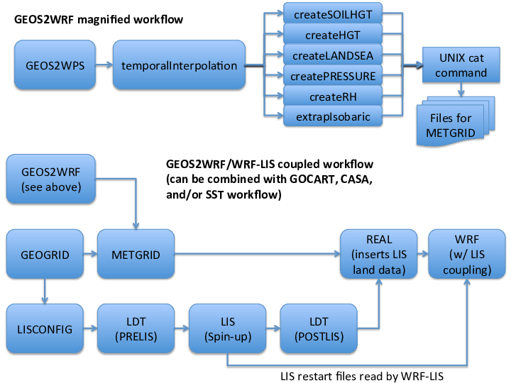
GEOS2WRF

GEOS2WRF can be broken down into four main sub-groups:

Front-end conversion.
- GEOS2WPS. A front-end converter that can read HDF4, netCDF3, and netCDF4 files with GEOS-5 data. A namelist.geos2wps file is read in as input, and must be customized to list the location, name, and format of the GEOS-5 file; the names of the coordinate arrays in the GEOS-5 file; the number of time slices, the indices of the slices, valid times and forecast hours; and the number of variables to process, along with their names, ranks, input and output names, units, and descriptions. This program takes the place of UNGRIB. The output from GEOS2WPS is written in WPS intermediate format [see Chapter 3 of NCAR 2022], with the filename convention $VARNAME_$LEVELTYPE:$YYYY-$MM-$DD_$HH, where $VARNAME is the variable name, $LEVELTYPE is a string describing the type of level the data are on, $YYYY is the 4-digit year, $MM is the 2-digit month, $DD is the 2-digit day, and $HH is the 2-digit hour. Some example output file names are:
  
  TT_MODEL_LEVEL:2009-08-25_00 # Temperature on model levels
  
  PSFC_GROUND_LEVEL:2009-08-25_00 # Surface pressure
  
  PMSL_MEAN_SEA_LEVEL:2009-08-25_00 # Mean sea level pressure
  
  VV_10M_ABOVE_GROUND_LEVEL:2009-08-25_00 # 10-meter V winds
  
  The $VARNAMEs (TT, PSFC, PMSL, and VV above) are listed in namelist.geos2wps, and can be customized by the user; however, they must match the values in the METGRID.TBL look-up file used by METGRID for those variables to be processed by WPS. (Intermediate variables used to derive other variables for WPS do not have this naming restriction.)
Temporal interpolation.
- temporalInterpolation. This program takes WPS intermediate file format data and linearly interpolates in time. This can be used, for example, to interpolate 6-hourly MERRA-2 analyses at 00Z, 06Z, 12Z, and 18Z to 3-hourly intervals for initializing WRF at 03Z, 09Z, 15Z, or 21Z. Only a single, user-specified variable will be processed during a particular program invocation, and other variables in the input data files will be ignored. A namelist.temporalInterpolation file is used to specify the variable, input, and output data files.
Variable-derivation. Multiple tools for deriving missing variables are required by WRF from existing variables. These should be used on an as-needed basis depending on the contents of the GEOS-5 files. Current programs that are in this category are:
- createSOILHGT. A utility that reads in a WPS file with surface geopotential, and calculates the surface terrain field. The output WPS file will be named SOILHGT_GROUND_LEVEL:$YYYY-$MM-$DD_$HH. A namelist.createSOILHGT file is also used as input.
- createHGT. A utility that reads in a WPS file with model layer pressure thicknesses, model layer temperatures, model layer specific humidity, and the model terrain field, and derives the geopotential heights on the GEOS-5 model levels. The output WPS files will be named HGT_MODEL_LEVEL:$YYYY-$MM-$DD_$HH. A namelist.createHGT file is also used as input. This program is not needed when processing isobaric levels.
- createLANDSEA. A utility that reads in a WPS file with “lake fraction” and “ocean fraction” and derives a land-sea mask. The output WPS files will be named LANDSEA_GROUND_LEVEL:$YYYY-$MM-$DD_$HH. A namelist.createLANDSEA file is also used as input.
- createPRESSURE. A utility that reads in a WPS file with model layer pressure thicknesses, and calculates the (mid-layer) pressures. The output WPS files will be named PRESSURE_MODEL_LEVEL:$YYYY-$MM-$DD_$HH. A namelist.createPRESSURE file is also used as input. This program is not needed when processing isobaric levels.
- createRH. A utility that reads in a WPS file with either model or isobaric level temperatures, specific humidity, and pressure, plus optional surface pressure, 2-meter temperature, and 2-meter specific humidity, and derives relative humidity on those levels. The output WPS files will have prefixes of RH_2M_ABOVE_GROUND_LEVEL, RH_MODEL_LEVEL, and/or RH_ISOBARIC_LEVEL, and will end with the familiar $YYYY-$MM-$DD_$HH string. A namelist.createRH file is also used as input. This program is recommended because some versions of REAL do not correctly interpolate specific humidity, and because the WRF definition of RH is strictly w.r.t. liquid while some versions of GEOS-5 output a weighted average of RT w.r.t. liquid and ice that is a function of temperature.
Extrapolation.
- extrapIsobaric. A utility that reads in a WPS file with geopotential height, temperature, relative humidity, U and V winds all on isobaric levels and extrapolates to those levels that are underground. The RH, U, and V nearest the ground are simply copied downward, while a specified lapse rate is used for temperature and the hypsometric equation is used for geopotential height. The output WPS files will be called ISOBARIC:$YYYY-$MM-$DD_$HH and will contain all the isobaric data (original data above ground, extrapolated data below ground.) A namelist.extrapIsobaric file is also used as input. This program is not necessary when processing GEOS-5 model-level data, since the GEOS-5 coordinate is terrain following. Users are advised to use the model-level data whenever possible.
Splitter utility.
- splitWPS. A utility that reads in a WPS file and divides the data into new WPS files, each file containing a single 2D slab of data. The output WPS files will be called $VARNAME_$LEVEL:$YYYY-$MM-$DD_$HH, where $LEVEL is the “level code” for the slab. The “level code” follows WPS convention: pressure levels are simply the pressure in Pa; model levels are the indices of the slice (“1” indicates model top in GEOS-5); ground level, 2-meter AGL, and 10-meter AGL are represented as “200100”; and the mean sea level is represented as “201300”. A namelist.splitWPS is also used as input. This program is not required for preparing data for WPS, but instead allows breaking up a WPS file into individual fields for examination.

To proceed, the user must first compile the GEOS2WRF software with ./build.sh geos2wrf. The user must then review the GEOS-5 data available to them and identify time slices and date/time stamps of interest, and the variables that can be used as-is by WRF. WRF will ultimately require the following fields on either isobaric or GEOS-5 model levels:

pressure;
geopotential height;
horizontal winds;
temperature; and
moisture (preferably relative humidity w.r.t. liquid).

Recommended fields that are useful for interpolating or extrapolating near the WRF model terrain level includes:

surface pressure;
sea level pressure;
land-sea mask;
sea-ice fraction;
2-m temperature;
2-m relative humidity;
10-m horizontal winds;
skin temperature; and
terrain height.

With this list in mind, the user must also identify GEOS-5 variables that can be used to derive other variables for WRF. From the utilities listed above, the following derivations can be made:

Surface geopotential can be used to derive terrain height (via createSOILHGT).
Lake fraction and ocean fraction can be used together to derive a land-sea table (via createLANDSEA).
Model layer pressure thicknesses can be used to derive model layer pressures (via createPRESSURE).
Model layer pressure thicknesses can also be used (with model layer temperatures, model layer specific humidity, and the model terrain field) to derive model layer geopotential heights (via createHGT).
Relative humidity on model levels, isobaric levels, and near ground level can be derived from model, isobaric, and 2-meter temperatures, model, isobaric, and 2-meter specific humidity, and model, isobaric, and surface pressure (via createRH).
Isobaric temperature, relative humidity, U and V winds can be extrapolated underground (via extrapISOBARIC).

After assembling the list of variables, the user should run GEOS2WPS using a customized namelist.geos2wps for each GEOS-5 file. Execution occurs with a simple ./geos2wps.x if in the current directory.

After extracting all the GEOS-5 variables, the user must employ the necessary utilities to derive the remaining variables for WRF. The appropriate namelist file (e.g., namelist.createHGT) must be customized, and the user must use the UNIX cat command to collect the relevant WPS files together. When ready, the user will execute by typing the program name (e.g., ./createHGT).

The namelist.geos2wps file contains the following information:

Variable Names	Description
&files
geosFileFormat	Integer, specifies GEOS-5 file format HDF4=1, netCDF3 or netCDF4 = 2, HDFEOS2=4
geosFileName	String, specifies GEOS-5 input file name to read.
outputDirectory	String, directory name to write WPS file.
&coordinates
longitudeName	String, name of 1-D longitude array in GEOS-5 file.
latitudeName	String, name of 1-D latitude array in GEOS-5 file.
hasVerticalDimension	Logical, specifies whether data with vertical dimension are to be processed from GEOS-5 file.
verticalName	String, name of 1-D vertical coordinate array in GEOS-5 file.
&forecast
numberOfTimes	Integer, number of time slices to process from GEOS-5 file.
validTimes(:)	Array of Strings, specifies valid time(s) of each time slice to process. Format is $YYYY-$MM-$DD_$HH. One array entry should exist for each time slice.
timeIndices(:)	Array of Integers, specifies time slice indices to process. One array entry should exist for each time slice.
forecastHours(:)	Array of Integers, specifies nominal forecast hour length for each processed time slice. One array entry should exist for each time slice.
&variables
numberOfVariables	Integer, specifies total number of variables to process from the GEOS-5 file.
variableRanks(:)	Array of Integers, specifies the ranks (number of dimensions) for each GEOS-5 variable to process. Data of rank 3 are assumed to be organized as (lat,lon,time), while rank 4 data are assumed to be organized as (lat,lon,vert,time). One array entry should be assigned for each processed variable.
variableLevelTypes(:)	Array of Integers, specifies level type for each processed variable. One array entry should be assigned for each variable. = 1, ground level; = 2, 2-meters AGL; = 3, 10-meters AGL = 4, mean sea level; = 11, model level; = 12, isobaric level
variableNamesIn(:)	Array of Strings, specifies the name of each processed variable in GEOS-5 file. One array entry should be specified for each variable.
variableNamesOut(:)	Array of Strings, specifies the name of each processed variable as written in the WPS file. One array entry should be specified for each variable. Not that if a processed variable is intended for direct use by WPS (instead of use in deriving something else), the variableNamesOut entry should match that in `METGRID.TBL` file used by METGRID.
variableUnits(:)	Array of Strings, specifies units of each processed GEOS-5 variable. One array entry should be specified for each variable. This is included because some GEOS-5 variables are known to be assigned the wrong units when output by the model.
variableDescriptions(:)	Array of Strings, gives short descriptions of each processed variable as written in the WPS file. One array entry should be specified for each variable.
&subsetData
subset	Logical, specifies whether to process the entire GEOS-5 domain or to read and process a subset.
iLonMin	Integer, specifies minimum i (longitude) index of GEOS-5 grid to process. Only used if subset=.true.
iLonMax	Integer, specifies maximum i (longitude) index of GEOS-5 grid to process. Only used if subset=.true.
jLatMin	Integer, specifies minimum j (latitude) index of GEOS-5 grid to process. Only used if subset=.true.
jLatMax	Integer, specifies maximum j (latitude) index of GEOS-5 grid to process. Only used if subset=.true.
kVertMin	Integer, specifies minimum k (vertical) index of GEOS-5 grid to process. Only used if subset=.true.
kVertMax	Integer, specifies maximum k (vertical) index of GEOS-5 grid to process. Only used if subset=.true.

The namelist.temporalInterpolation file contains the following information:

Variable Names	Description
&all
fieldName	String, lists name of the variable to process.
&input1
directory1	String, lists directory with WPS intermediate file.
prefix1	String, lists prefix of the name of WPS intermediate file.
year1	Integer, lists the valid year of the WPS intermediate file.
month1	Integer, lists valid month of WPS intermediate file.
day1	Integer, lists the valid day of the WPS intermediate file.
hour1	Integer, lists valid hour of WPS intermediate file.
&input2
directory2	String, lists directory with WPS intermediate file.
prefix2	String, list prefix of the name of WPS intermediate file.
year2	Integer, lists the valid year of the WPS intermediate file.
month2	Integer, lists valid month of WPS intermediate file.
day2	Integer, lists the valid day of the WPS intermediate file.
hour2	Integer, lists valid hour of WPS intermediate file.
&output
directoryOutput	String, lists directory with WPS intermediate file.
prefixOutput	String, lists prefix of the name of WPS intermediate file.
yearOutput	Integer, lists the valid year of the WPS intermediate file.
monthOutput	Integer, lists valid month of WPS intermediate file.
dayOutput	Integer, lists the valid day of WPS intermediate file.
hourOutput	Integer, lists valid hour of WPS intermediate file.

The namelist.createSOILHGT file contains the following information:

Variable Names	Description
&input
directory	String, directory for input and output WPS files.
prefix	String, lists filename prefix of input WPS files.
year	Integer, lists valid year of WPS file.
month	Integer, lists valid month of WPS file.
day	Integer, lists valid day of WPS file.
hour	Integer, lists valid hour of WPS file.
surfaceGeopotentialName	String, name of the surface geopotential field in WPS file

The namelist.createHGT file contains the following information:

Variable Names	Description
&input
directory	String, directory for input and output WPS files.
prefix	String, lists filename prefix of input WPS files.
year	Integer, lists the valid year of the WPS file.
month	Integer, lists valid month of WPS file.
day	Integer, lists the valid day of the WPS file.
hour	Integer, lists valid hour of the WPS file.
layerPressureThicknessName	String, name of pressure thickness variable between GEOS-5 model levels in the input WPS file.
layerTemperatureName	String, name of model layer temperatures in the input WPS file.
layerSpecificHumidityName	String, name of model layer specific humidity variable in the input WPS file.
soilHeightName	String, name of surface terrain variable in the input WPS file.
modelTopPressure	Real, air pressure (in PA) at the very top of GEOS-5 grid. For GEOS-5, this is typically 1 Pa (0.01 mb).

The namelist.createLANDSEA file contains the following information:

Variable Names	Description
&input
directory	String, directory for input and output WPS files.
prefix	String, lists filename prefix of input WPS files.
year	Integer, lists the valid year of the WPS file.
month	Integer, lists valid month of WPS file.
day	Integer, lists the valid day of the WPS file.
hour	Integer, lists valid hour of the WPS file.
lakeFractionName	String, name of the GEOS-5 variable specifying fraction of grid point covered by lakes in the WPS input file.
oceanFractionName	String, GEOS-5 variable name specifying fraction of grid point covered by the ocean in the WPS input file.

The namelist.createPRESSURE file contains the following information:

Variable Names	Description
&input
directory	String, directory for input and output WPS files.
prefix	String, lists filename prefix of input WPS files.
year	Integer, lists the valid year of the WPS file.
month	Integer, lists valid month of WPS file.
day	Integer, lists the valid day of the WPS file.
hour	Integer, lists valid hour of the WPS file.
layerPressureThicknessName	String, names variable with pressure thicknesses between GEOS model levels in the WPS input file.
modelTopPressure	Real, air pressure (in PA) at very top of GEOS-5 grid. For GEOS-5, this is typically 1 Pa (0.01 mb).

The namelist.createRH file contains the following information:

Variable Names	Descriptions
&input
directory	String, lists directory for input and output WPS files
prefix	String, lists filename prefix of input WPS files.
year	Integer, lists the valid year of the WPS file.
month	Integer, lists valid month of WPS file.
day	Integer, lists the valid day of the WPS file.
hour	Integer, lists valid hour of the WPS file.
processSurfacePressure	Logical, indicates whether or not to read in surface pressure from the WPS input file.
onIsobaricLevels	Logical, indicates whether upper air levels are isobaric instead of model level.
surfacePressureName	String, name of surface pressure variable in WPS input file. Ignored if processSurfacePressure=.false.
pressureName	String, name of upper-level pressure fields in WPS input file. Ignored if onIsobaricLevels=.true.
temperatureName	String, name of temperature fields in WPS input file If 2-meter temperatures are included, then the surface pressure must also be supplied and processSurfacePressure must be set to .true.
specificHumidityName	String, name of specific humidity fields in WPS input file. If 2-meter specific humidities are included, then the surface pressure must also be supplied and processSurfacePressure must be set to .true.

The namelist.extrapIsobaric file contains the following information:

Variable Names	Description
&input
directory	String, lists directory for input and output WPS files
prefix	String, lists filename prefix of input WPS files.
year	Integer, lists the valid year of the WPS file.
month	Integer, lists valid month of WPS file.
day	Integer, lists the valid day of the WPS file.
hour	Integer, lists valid hour of the WPS file.
geopotentialHeightName	String, name of isobaric geopotential height fields in the WPS input file.
temperatureName	String, name of isobaric temperature fields in the WPS file.
relativeHumidityName	String, name of isobaric relative humidities in the WPS input file.
uName	String, name of isobaric zonal wind field in WPS input file.
vName	String, name of isobaric meridional wind field in WPS input file.

The namelist.splitWPS file contains the following information:

Variable Names	Description
&input
directory	String, lists directory for input and output WPS files.
prefix	String, lists filename prefix of input WPS files.
year	Integer, lists the valid year of the WPS file.
month	Integer, lists valid month of WPS file.
day	Integer, lists the valid day of the WPS file.
hour	Integer, lists valid hour of the WPS file.

A sample script (utils/geos2wrf/scripts/merra/run_geos2wrf_merra2_3hrassim.sh) is available to use GEOS2WRF to process 3-hourly MERRA-2 assimilation data. These data are output from GEOS-5 when the global model is adjusting toward a MERRA-2 6-hourly analysis via Incremental Analysis Updates [see section 4.2 of Rienecker et al. (2008)]. This script will run GEOS2WPS, createLANDSEA, createSOILHGT, and createRH to process the data. To run, the user must edit the accompanying config.discover.sh file to set the path to the NU-WRF code, the work directory, and the modules used to compile GEOS2WRF; then, the run_geos2wrf_merra2_3hrassim.sh should be modified to specify the start and end dates and hours to process. (Users who wish to use 6-hourly MERRA or MERRA-2 data can use either GEOS2WRF or MERRA2WRF; however, the 3-hourly MERRA-2 data can only be processed with GEOS2WRF.)

MERRA2WRF

MERRA2WRF is a monolithic program customized to process the 6-hourly reanalyses from MERRA and MERRA-2. It was first developed for MERRA under the assumption that the archived data files (called “collections” in GEOS-5 terminology) would be permanent, making it possible to build a single robust preprocessing tool. Recently support was added for 6-hourly MERRA-2 fields; however, 3-hourly MERRA-2 processing is not possible due to significant differences in the data collections (users must fall back to GEOS2WRF for these 3-hourly data).

MERRA and MERRA-2 files are accessible from the NASA GES DISC web page (http://disc.sci.gsfc.nasa.gov), and are available to the general public. MERRA-2 files are also accessible on the NASA Discover supercomputer in /discover/nobackup/projects/gmao/merra2/merra2/scratch/ but are only available to select users authorized by the GMAO.

MERRA2WRF is compiled when running ./build.sh geos2wrf. The following files must then be gathered from the MERRA or MERRA-2 datasets:

const_2d_asm_Nx (in HDFEOS2 or NETCDF format):
- ’XDim’ or ’lon’ (longitude)
- ’YDim’ or ’lat’ (latitude)
- ’PHIS’ (surface geopotential)
- ’FRLAKE’ (lake fraction)
- ’FROCEAN’ (ocean fraction)
inst6_3d_ana_Nv (variable names are HDF4 or netCDF or HDFEOS2):
- ’longitude’ or ’XDim’ or ’lon’ (longitude)
- ’latitude’ or ’YDim’ or ’lat’ (latitude)
- ’time’ or ’TIME:EOSGRID’ or ’TIME’ (synoptic hour)
- ’levels’ or ’Height’ or ’lev’ (nominal pressure for each model level)
- ’ps’ or ’PS’ (surface pressure)
- ’delp’ or ’DELP’ (layer pressure thicknesses)
- ’t’ or ’T’ (layer temperature)
- ’u’ or ’U’ (layer eastward wind)
- ’v’ or ’V’ (layer northward wind)
- ’qv’ or ’QV’ (layer specific humidities)
inst6_3d_ana_Np (variable names are HDF4 or netCDF or HDFEOS2):
- ’longitude’ or ’XDim’ or ’lon’ (longitude)
- ’latitude’ or ’YDim’ or ’lat’ (latitude)
- ’time’ or ’TIME:EOSGRID’ or ’TIME’ (synoptic hours)
- ’slp’ or ’SLP’ (sea level pressure)
tavg1_2d_slv_Nx (variable names are HDF4 or netCDF or HDFEOS2):
- ’longitude’ or ’XDim’ or ’lon’ (longitude)
- ’latitude’ or ’YDim’ or ’lat’ (latitude)
- ’time’ or ’TIME:EOSGRID’ or ’TIME’ (synoptic hours)
- ’u10m’ or ’U10M’ (10-meter eastward wind)
- ’v10m’ or ’V10M’ (10-meter northward wind)
- ’t2m’ or ’T2M’ (2-meter temperature)
- ’qv2m’ or ’QV2M’ (2-meter specific humidity)
- ’ts’ or ’TS’ (skin temperature)
tavg1_2d_ocn_Nx (variable names are HDF4/netCDF or HDFEOS2):
- ’longitude’ or ’XDim’ or ’lon’ (longitude)
- ’latitude’ or ’YDim’ or ’lat’ (latitude)
- ’time’ or ’TIME:EOSGRID’ or ’TIME’ (synoptic hours)
- ’frseaice’ or ’FRSEAICE’ (sea ice fraction)
tavg1_2d_lnd_Nx (variable names are HDF4/netCDF or HDFEOS2):
- ’longitude’ or ’XDim’ or ’lon’ (longitude)
- ’latitude’ or ’YDim’ or ’lat’ (latitude)
- ’time’ or ’TIME:EOSGRID’ or ’TIME’ (synoptic hours)

Note that the tavg1_2d_*_Nx collections are 1-hour averages that are valid at the bottom of the hour. For simplicity, MERRA2WRF uses the 00:30Z average data with the 00Z instantaneous fields, the 06:30Z average data with the 06Z instantaneous fields, and so on.

To download the MERRA data and run MERRA2WRF for a specified start date and end date go to scripts/python/utils and run merra2wrf.py using the command:

./merra2wrf.py StartDate EndDate -o OutputDir -n NUWRFDIR.

For example:

./merra2wrf.py 20150711 20150712 -n <NUWRFDIR>
Start MERRA2WRF conversion...
start_time: 20150711
end_time:   20150712
out_dir:    ./
nuwrf_dir:  <NUWRFDIR>
date:  2015 07 11
getting files...
running merra2wrf...
date:  2015 07 12
getting files...
running merra2wrf...
Time taken = 110.273767
./merra2wrf.py is DONE.

A namelist file will be created for each processing date, and files readable for METGRID will be generated in a data directory under out_dir.

To use MERRA-2 reanalysis, the user may download MERRA-2 files from the GES DISC web page and process them with MERRA2WRF got to the utils/geos2wrf/scripts/run_merra directory and run:

./proc_merra2_ges_disc.sh StartDate EndDate RunDir NUWRFDIR

A third alternative is to customize namelist.merra2wrf by hand to process the selected MERRA files and namelist.merra2_2wrf to process the selected MERRA-2 files (both files are in utils/geos2wrf/namelist). The namelist files consist of a single block:

Variable Names	Description
&input
outputDirectory	String, lists directory for writing WPS output files.
merraDirectory	String, lists directory containing MERRA or MERRA-2 input files.
merraFormat_const_2d_asm_Nx	Integer, specifies format of const_2d_asm_Nx file. 1=HDF4, 2=netCDF, 4=HDFEOS2.
merraFile_const_2d_asm_Nx	String, name of const_2d_asm_Nx file.
numberOfDays	Integer, lists number of days to process. Each MERRA or MERRA-2 collection (excluding const_2d_asm_Nx) will have one file per day.
merraDates(:)	Array of strings, list each day to be processed (format is YYYY-MM-DD).
merraFormat_inst6_3d_ana_Nv	Integer, specifies format of inst6_3d_ana_Nv files. 1=HDF4, 2=netCDF, 4=HDFEOS2.
merraFiles_inst6_3d_ana_Nv(:)	Array of strings, specifying names of inst6_3d_ana_Nv files.
merraFormat_inst6_3d_ana_Np	Integer, specifies format of inst6_3d_ana_Np files. 1=HDF4, 2=netCDF, 4=HDFEOS2.
merraFiles_inst6_3d_ana_Np(:)	Array of strings, specifying names of inst6_3d_ana_Np files.
merraFormat_tavg1_2d_slv_Nx	Integer, specifies format of tavg1_2d_slv_Nx files. 1=HDF4, 2=netCDF, 4=HDFEOS2.
merraFiles_tavg1_2d_slv_Nx(:)	Array of strings, specifying names of tavg1_2d_slv_Nx files.
merraFormat_tavg1_2d_ocn_Nx	Integer, specifies format of tavg1_2d_ocn_Nx files. 1=HDF4, 2=netCDF, 4=HDFEOS2.
merraFiles_tavg1_2d_ocn_Nx(:)	Array of strings, specifying names of tavg1_2d_ocn_Nx files.

The software is run by typing ./merra2wrf.x namelist.merra2wrf. The output files will be named MERRA:$YYYY-$MM-$DD_$HH, where $YYYY is the four-digit year, $MM is the two-digit month, $DD is the two-digit day, and $HH is the two-digit hour. These files are readable by METGRID.

Use of New Erodible Soil Options

NU-WRF includes several new options for specifying erodible soil (EROD) for dust emissions (Kim, Kemp, and Chin 2014). The workflow depends a bit on the particular option selected but requires compilation of WRF-Chem and WPS (./build.sh chem,wps if using normal chemistry, or ./build.sh kpp,wps if using KPP chemistry).

The four available EROD options are:

EROD_STATIC. This is the EROD option inherited from the community WRF. Annual EROD at 0.25 deg resolution for sand, silt, and clay is processed and fed to WRF-Chem.
EROD_MDB. This is a new seasonal EROD dataset derived from MODIS-Deep Blue climatological aerosol products. [See Ginoux et al. (2012) and Ginoux et al. (2010) for description of estimating frequency of occurrance of optical depth – these are converted to EROD]. Data are subdivided into three groups (for sand, silt, and clay) at 0.1 deg resolution for four meteorological seasons (December-January-February, March-April-May, June-July-August, September-October-November). These are processed and passed to WRF-Chem.
EROD_DYN_CLIMO. This is a new “dynamic climatological” EROD option. It uses a monthly surface bareness field derived at 30-arc second resolution from the community WRF climatological MODIS vegetation fraction dataset (greenness_fpar_modis/), with adjustments from the community WRF’s soil type and MODIS and USGS land use datasets to screen out water bodies. It also uses a 30-arc second topographic depression dataset derived from the community WRF’s terrain dataset. These fields are passed to WRF-Chem, which will create an instantaneous EROD field from these variables with adjustments to screen out snowy or very cold locations.
EROD_DYN. This is a new “dynamical” EROD option. It uses the same topographic depression field as EROD_DYN_CLIMO, plus a surface bareness field based on either NASA GIMMS or NASA SPoRT daily NDVI products. The data are passed to WRF-Chem, which will construct an instantaneous EROD field from the bareness and topographic depression with adjustments to screen out snowy or very cold locations.

A sample workflow for EROD is presented here:

Assemble GEOG data. Several new EROD-related fields must be obtained from the NU-WRF group and placed in subdirectories with the standard GEOG data available from the community WRF. For EROD_MDB, they are erod_mdb_clay_0.1deg/, erod_mdb_sand_0.1deg/, and

erod_mdb_silt_0.1deg/. For EROD_DYN_CLIMO, they are

bareness_dyn_climo/ and TOPODEP_30s/. For EROD_DYN, the TOPODEP_30s/ data must be staged; in addition, the user is advised to collect NDVI-based greenness in GEOGRID format from NASA SPoRT and place the files in a gvfsport/ directory.
Create NDVI-based bareness for EROD_DYN option. The NDVIBARENESS4WRF tool is used to process NDVI data and generate a bareness field. Both bareness and NDVI are written in WPS intermediate format for direct ingest into METGRID. The NDVIBARENESS4WRF code is described by Kemp (2016).
GEOGRID. Run for terrestrial processing. Use the GEOGRID.TBL.ARW_CHEM_NUWRF file to ensure EROD-related fields are specified. If preparing for the EROD_DYN option, “gvfsport” should be specified as the first part of the “geog_data_res” option in namelist.wps – this will ensure the SPoRT greenness is processed rather than the climatological greenness data available with the community WRF.
UNGRIB. Run for normal GRIB file processing.
METGRID. Run for normal processing. If preparing for the EROD_DYN option, user should modify namelist.wps to include the file prefix(es) for the bareness data in the “fg_name” namelist option. Note that the METGRID.TBL.ARW file in NU-WRF has been modified to recognize the new EROD-related fields.
REAL. Run to produce initial and lateral boundary conditions. Namelist variable “chem_opt” should be set to 401 for simple dust treatment. (Dust emissions can also be used with GOCART chemistry by setting “chem_opt” to 300, 301, 302, or 303; however, in this case, the workflow must be expanded to include the steps in Use of GOCART Aerosol Data.) New namelist variable “erod_option” in the &chem block should be set to “static”, “mdb”, “dyn_climo”, or “dyn”. If not set, “static” is assumed.
WRF. Run for EROD simulation. Optionally set the new “gocart_dustemiss_layer” namelist variable to highest vertical model level to spread dynamic dust (default is 1), or set “gocart_dustemiss_suppress=1” to shut off dynamic dust emissions. The new variable EROD_TIMESTEP in the wrfout netCDF file will show the instantaneous EROD field for sand, silt, and clay for whatever EROD option is used. Other variables of note are:
- BARENESS_DYN_CLIMO: Monthly input bareness field for
  
  EROD_DYN_CLIMO option.
- EROD_MDB_CLAY: Seasonal EROD for clay for EROD_MDB option.
- EROD_MDB_SAND: Seasonal EROD for sand for EROD_MDB option.
- EROD_MDB_SILT: Seasonal EROD for silt for EROD_MDB option.
- EROD_STATIC: The standard EROD field available with the community WRF.
- TOPODEP: The topographic depression values for sand, silt, and clay for the EROD_DYN_CLIMO and EROD_DYN options.

Use of GOCART Aerosol Data

NU-WRF offers advanced aerosol modeling using the implementation of GOCART [see Chin et al. (2002) and Ginoux et al. (2001)] in WRF-Chem. Running GOCART in WRF allows for aerosol coupling with the Goddard 4ICE microphysics scheme and with the 2017 Goddard radiation scheme, providing a simulation of the direct and indirect aerosol effects on weather and climate. For best results, it is necessary to provide initial and lateral boundary conditions for GOCART, plus surface-based emissions. To that end, the NU-WRF modeling system includes the new GOCART2WRF preprocessor for providing chemical boundary conditions from the GEOS-5, and includes the community PREP_CHEM_SOURCES program for emissions. To run, the user must compile with

./build.sh chem,wps,gocart2wrf,prep_chem_sources,plot_chem.

GOCART2WRF supports four possible sources of GOCART data:

offline GOCART;
on-line GOCART from GEOS-5;
MERRAero reanalyses Kishcha et al. (2014); and
MERRA-2 `Bosilovich et al. (2015) <#bosi>`__reanalyses.

A workflow supporting the use of GOCART in NU-WRF might look like this:

WPS. Perform terrestrial and meteorological preprocessing as normal.
REAL. Generate meteorological initial and lateral boundary conditions as normal.

GOCART2WRF. Process GOCART data and insert into output files from REAL. Typically the user must edit a namelist.gocart2wrf to specify the number of WRF domains, the location of REAL output files, and the location, source, and file prefixes of the GOCART files. GOCART2WRF is then executed at the command line using ./gocart2wrf with namelist.gocart2wrf in the current working directory. GOCART2WRF will obtain the required dates and times from the REAL netCDF files, search the GOCART files for the corresponding dates and times, read and interpolate the required GOCART variables, and essentially append those fields to the REAL files. Currently, 17 GOCART variables are processed: Hydrophobic and Hydrophilic Black Carbon, Hydrophobic and Hydrophilic Organic Carbon, dust particles with 0.5 $μ$ m, 1.4 $μ$ m, 2.4 $μ$ m, 4.5 $μ$ m, and 8.0 $μ$ m effective radii, sea salt particles with 0.3 $μ$ m, 1.0 $μ$ m, 3.2 $μ$ m, and 7.5 $μ$ m effective radii, and concentrations of Dimethyl Sulfide, Methanesulfonic Acid, Sulfur Dioxide, and Sulfate.

The namelist.gocart2wrf file contains the following entries:

Variable Names	Description
&wrf
max_dom	Integer, specifies number of WRF domains.
wrf_dir	String, specifies directory with wrfinput and wrfbdy files.
&gocart_shared
gocart_format	Integer, specifies format of GOCART data; currently must be set to 5 (for netCDF4 files)
gocart_source	String, lists source of GOCART data. 4 options are available: ’GEOS’ : Output from GEOS-5 (default) ’MERRA2’ : Output from MERRA-2 reanalysis ’MERRAERO’ : Output from MERRAero reanalysis ’OFFLINE’ : Output from offline GOCART
gocart_dir	String, specifies directory with netCDF4 GOCART files to process. If processing MERRAero or MERRA2 data, files are assumed to be in subdirectories, e.g., For MERRAERO: `gocart_dir/Y2005/M05/` For MERRA-2: `gocart_dir/$STREAM/stage/Y2005/M05/` where $STREAM is MERRA2_100 for data before 1992, MERRA2_200 for data from 1992 to 2000, MERRA3_300 for data from 2001 to 2010, or MERRA2_400 for data from 2011 on.
gocart_prefix	String, specifies file name prefix for netCDF4 GOCART files. Ignored if processing MERRA-2 or MERRAero data.

If processing MERRA-2 data, the user can download MERRA-2 GOCART files from the GES DISC web page, and process them with GOCART2WRF. The command is:

./proc_merra2_gocart_ges_disc.sh NumDomains StartDate EndDate RunDir NUWRFDIR

A namelist file will be created by the script and updated wrfbdy_d01 and wrfinput_d* netCDF files will be created.

PREP_CHEM_SOURCES. This community tool processes a number of biogenic, anthropogenic, volcanic, and wildfire emissions Freitas et al. (2011). Operating this program is largely described in Peckham et al. (2015) and Peckham et al. (2022), and requires customizing a prep_chem_sources.inp file and downloading emissions data supported by the program. The NU-WRF version has several modifications:
- Map projection. The map projection code from WPS has been added to PREP_CHEM_SOURCES to ensure consistency in emission interpolation. This support is automatic when using the NU-WRF build system, and no user action is required.
- Improved GOCART background fields. Processing emissions for GOCART requires monthly climatological background fields of Hydrogen Peroxide, Hydroxide, and Nitrate. The community data for PREP_CHEM_SOURCES contains 55 vertical levels, is only for 2006, and is missing some information useful for vertical interpolation. New 72-level datasets produced by GSFC are now available in two formats with improved vertical interpolation information. The user should edit prep_chem_sources.inp and set use_gocart_nuwrf=1 and “gocart_nuwrf_data_type” variable to “old” or “new” to switch between the community and new files. If “new” files are selected, they must be in a gocart_nuwrf_data_dir subdirectory on the same level as the gocart_bg/ folder containing the community 55-level files. If “new” is selected, the program will first search for geos5_met_1MAVG_YYYYMM.nc and gmi_merra_oxidants_YYYYMM_1.25x1.nc files, where YYYY is the 4-digit year and MM is the 2-digit month. If the program fails to find both files, it will fall back on gmi_2006MM.nc files, which are also new 72-level files but only exist for 2006.
- Improved interpolation of GOCART background fields. The community PREP_CHEM_SOURCES program uses simple averaging of GOCART background grid points to each WRF grid point, which implicitly assumes the WRF grid is at a coarser resolution than the background. This results in unphysical blocky fields, which are further marred by gradients associated with sharp WRF terrain. In the NU-WRF version of PREP_CHEM_SOURCES, bilinear interpolation is used in cases where less than two background grid points are averaged to a WRF grid point, leading to much smoother fields.
- GFEDv4. The GFEDv4 biomass burning emissions dataset [Randerson et al. (2015)] is supported. It supersedes and replaces the Global Fire Emissions Database, Version 3.1 (GFEDv3.1). To use it the user must edit the prep_chem_sources.inp file, toggle the new variable “use_gfedv4=1”, set the new “gfedv4_data_dir” variable to specify the directory with the GFEDv4 data, and edit the new “gfedv4_suffix” variable to list the species to process. There are sample prep_chem_sources.inp files in the scripts/regression/testcases/chem directories with default settings for the DISCOVER system. Note that GFEDv4 and other GFED data sets cannot be used simultaneously. Currently the following species can be processed: BC, C2H4, C2H4O, C2H4, C2H5OH, C2H6S, C2H6, C3H6O, C3H6, C3H8, CH4, C5H8, CH2O, CH3OH, CH4, CO2, CO, NH3, NOx, OC, PM2p5, SO2, Terpenes, Toluene_lump, and TPM. DM can also be processed but is not currently used by WRF-Chem.
- QFED. The NASA QFED wildfire emissions dataset [Darmenov and da Silva (2013)] is supported. The user must edit the prep_chem_sources.inp file, toggle the new variable “use_qfed=1”, set the new “qfed_data_dir” variable to specify the top directory with QFED data (yearly subdirectories like Y2005/ are assumed, with monthly subdirectories like M05/ within each annual subdirectory), and edit the new “qfed_suffix” variable to list the species to process (e.g, “bc,oc,pm25,so2”). Note that the species are used to construct the names of the emissions files (e.g, qfed2.emis_bc.005.20140404.nc4, so the names are case sensitive. Also, note that QFED cannot be used simultaneously with GFED source options. Currently, the following QFED species can be processed: acet, ald2, alk4, bc, c2h6, c3h6, c3h8, ch2o, ch4, co, co2, mek, nh3, no, oc, pm25, and so2.
- Output of map projection data. New .map files with map projection data are automatically output. These files are intended for use by PLOT_CHEM to visualize the fields.
PLOT_CHEM. This is an optional step to create simple visualizations of emissions output from PREP_CHEM_SOURCES. The program reads in a GrADS control file produced by PREP_CHEM_SOURCES, the corresponding GrADS binary file, and the special .map file with critical map projection information. PLOT_CHEM will then create visualizations of each field using NCAR Graphics. The plots are not publication quality and are only intended for sanity checking. To run, the user must first create a symbolic link grads.ctl to the desired GrADS control file, and then run ./plot_chem in the same directory as the GrADS and .map files. The output is a gmeta file which can be viewed using the NCAR Graphics idt program (see http://ngwww.ucar.edu for information on NCAR Graphics).
CONVERT_EMISS. This is a community WRF-Chem preprocessor that takes the output from PREP_CHEM_SOURCES and rewrites the fields in new netCDF files for reading by WRF-Chem. This program is described in Peckham et al. (2015) and Peckham et al. (2022), and requires modifying a namelist.input file to specify domain information, physics, and chemistry options. The program is then run in the same directory as the namelist.input and the PREP_CHEM_SOURCES output files.

There are two issues to keep in mind:
- First, CONVERT_EMISS does not currently process more than one domain at a time. Thus, the user must process each domain in separate executions, and must rename the input files to use “d01” before execution, regardless of what the actual domain number is. The output files must then be renamed to restore the actual domain numbers for WRF-Chem. In addition, a namelist.input file must be customized for each execution with the “max_dom” variable set to “1” and the first grid domain variables (e.g., “dx”, “nx”, etc) conforming to whichever domain is being processed.
- Second, the output files from PREP_CHEM_SOURCES must be renamed to conform to the naming convention expected by CONVERT_EMISS. The naming convention for the different emissions files is documented in Peckham et al. (2015).
Note that if PREP_CHEM_SOURCES processed “new” GOCART background files, the &chem block in namelist.input must be modified to add “gocart_nuwrf_type=1” so CONVERT_EMISS will read 72 levels of data and perform the correct vertical interpolation. If this setting is omitted, the background fields output by CONVERT_EMISS will likely contain unphysical values. For ‘old’’ GOCART background files set “gocart_nuwrf_type=0”
WRF-Chem. Running WRF-Chem is similar to the Basic Workflow case, but requires the &chem namelist block to be included in the namelist.input with GOCART activated (chem_opt = 300, 301, 302, or 303). Aerosol coupling with the Goddard 4ICE schemes (mp_physics=7) will be activated if the new “gsfcgce_gocart_coupling” namelist variable is set to 1 (set by default). Likewise, aerosol coupling with the 2017 Goddard radiation schemes (ra_lw_physics=5 and ra_sw_physics=5) will be activated if the new “gsfcrad_gocart_coupling” namelist variable is set to 1 (set by default).

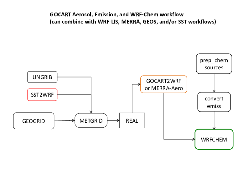
Use of CASA CO $_{2}$ Data

NU-WRF has the capability for running simulations with CO $_{2}$ treated as a tracer (i.e., no interaction with physics). This requires specifying initial, lateral boundary, and flux emission fields of CO $_{2}$ . To that end, several utilities have been written to process CASA global climatological CO $_{2}$ concentrations and flux emissions and provide them to WRF-Chem: READ_CO2_CONC, READ_CO2_FLUX, and CASA2WRF.

A particular capability of the CASA2WRF utility allows for the temporal interpolation of CASACO2 flux depending on the NU-WRF model state. This capability can be turned on by modifying the namelist.casa2wrf file and setting the “flux_interpolate” namelist variable equal to 1. With this option, the NU-WRF model state is read by CASA2WRF every hour and wrf-domain interpolated CO $_{2}$ flux components from 6 different sources

Respiratory (monthly)
Net Production (monthly)
Bio-fuel (monthly)
Fossil Fuel (yearly)
Wild fire (daily)
Ocean CO $_{2}$

are combined to produce total flux and flux tendency netCDF files that can be input to NU-WRF WRF-Chem runs.

To compile, the user must type ./build.sh casa2wrf. It creates the following executables in utils/bin:

Read_CO2_conc.x: Reads and converts a CO $_{2}$ concentration data file to netCDF format usable by NU-WRF.
Read_CO2_Flux.x: Reads and converts a CO $_{2}$ flux data file to netCDF format usable by NU-WRF.
ConvertData2Netcdf.x: Converts CO $_{2}$ flux component files in binary format to netCDF format.
casa2wrf.x: Processes and incorporates the CO $_{2}$ concentration and flux data to wrfinput_d*, wrfbdy_d01, and flux input files suitable for WRF-Chem runs.

Instructions for running these programs, including namelist definitions, are provided in Tao et al. (2014). A sample workflow is provided below:

WPS. Perform terrestrial and meteorological preprocessing as normal.
REAL. Generate meteorological initial and lateral boundary conditions as normal.
READ_CO2_CONC. Reads the CASA CO $_{2}$ concentration files in flat binary format, and converts to netCDF with a time stamp.
READ_CO2_FLUX. Reads the CASA CO $_{2}$ flux files in flat binary format, and converts to netCDF with a time stamp.
ConvertData2Netcdf. Reads the CASA CO $_{2}$ flux files from different sources in flat binary format, and converts to netCDF with a time stamp.
CASA2WRF. Read the CO $_{2}$ netCDF files, interpolates concentration and flux data to the WRF grids (single or nested), read the wrfout* files from a NU-WRF run every hour or any specified time interval from namelist, temporally interpolate the NPP and RESP CO $_{2}$ fluxes with relation the NU-WRF state, combine the fluxes from all sources, calculates the rates of change of flux/hour at the user specified time frequency, appends the interpolated concentrations to the initial and lateral boundary condition netCDF files (wrfinput_* and wrfbdy_d01), and writes the interpolated fluxes to a new netCDF file (CO2_domain_date).
WRF-Chem. Run WRF-Chem with CASA CO $_{2}$ chemistry options in the namelist.input (including chem_opt = 18, emiss_opt=18, and emiss_inpt_opt=18). Other appropriate settings are listed in Tao et al. (2014).

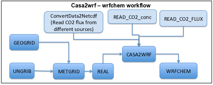
Use of SPoRT Sea Surface Temperature Data

NASA SPoRT generates sea surface temperature analyses for the northern western hemisphere every 12 hours valid at 06Z and 18Z. A script

fetch_sport_sst_northwestHemi.py is available to download GRIB2 files of these analyses from the SPoRT FTP site. The script and companion configuration file sport_sst_northwestHemi.cfg are in the scripts/python/utils/ directory. The configuration file specifies the start and end dates and hours for downloading data, along with the top directory for storing the downloaded files. The user can override the date/time information in this file by running fetch_sport_sst_northwestHemi.py with a -L flag (or equivalently, --latest) on the command line; this will cause the script to fetch all available files valid for the most recent 24 hours. Files will be uncompressed via gunzip after being downloaded.

The uncompressed GRIB2 files can be processed by UNGRIB (we recommend using the prefix “SPORT_SST” for the output files). The user must then edit the namelist.wps file to include the SPoRT SST prefix in the “fg_name” namelist variable so METGRID processes the data along with other atmospheric fields. When run, METGRID will replace the SST or skin temperature from atmospheric fields with that from the SPoRT analysis. The remaining steps (REAL and WRF) can be completed as normal.

Use of RSS Sea Surface Temperature Data

A special preprocessor included with NU-WRF is SST2WRF, which processes several sea surface temperature (SST) products produced by Remote Sensing Systems (RSS; see http://www.remss.com). These products are potential alternatives to the SST or skin temperature fields often provided in meteorological GRIB files (e.g., from the NOAA GFS or NAM models). Because RSS products are not available in GRIB format, UNGRIB cannot process them and a tool like SST2WRF is required as a substitute.

SST2WRF currently supports several different analysis products classified by source instrument and by algorithm version. The instrument SST analyses are

mw_ir. 9-km global SST valid at 1200 UTC based on microwave (TMI, AMSR-E, AMSR2, WindSat) and Infrared (Terra MODIS, Aqua MODIS) data.
mw. 25-km global SST valid at 0800 LT, based on Microwave (TMI, AMSR-E, AMSR2, WindSat) data.

The algorithm versions are:

rt. The real-time algorithm.
v04.0. Version 4 algorithm.

See http://data.remss.com/sst for a description of these products.

A workflow for SST2WRF could be similar to that in the Basic Workflow, but would require running SST2WRF in addition to UNGRIB. UNGRIB is responsible for processing meteorological fields, while SST2WRF will process only the SST related fields from RSS. (One could also replace UNGRIB with GEOS2WRF or MERRA2WRF; for simplicity, we will assume UNGRIB is used.)

The user must compile using ./build.sh sst2wrf. A script provided in

scripts/python/utils/sst2wrf.py can be used to download SST data. Run, ./sst2wrf -h to help set the required variables and fetch the data. For example:

./sst2wrf.py 20150711 20150712 -n <NUWRFDIR>
Start SST2WRF conversion...
start_time: 20150711
end_time:   20150712
inst_type:  mw_ir
data_vers:  v5
out_dir:    ./
nuwrf_dir:  <NUWRFDIR>
getting files for day # 192
running sst2wrf...
getting files for day # 193
running sst2wrf...
Time taken = 13.565437
./sst2wrf.py is DONE.

As an alternative, the user can customize a sample namelist file given in

utils/sst2wrf/namelist/namelist.sst2wrf to provide the following information:

Variable Names	Description
&input
instrument	String, specifies instrument(s) used for analysis; options are “mw_ir”, “mw”.
year	Integer, specifies valid year of analysis.
dayOfYear	Integer, specifies valid day of year of analysis.
version	String, specifies algorithm for analysis; options are “rt”,”v04.0”.
inputDirectory	String, specifies directory with SST file.
&output
outputDirectory	String, specifies directory for output file.
prefixWPS	String, specifies file name prefix for output; prefix must also be in `METGRID.TBL` for METGRID to process.
&fakeoutput
numFakeHours	Integer, specifies number of hours of each day that additional WPS files should be written for. Currently only one SST analysis is available per day, but METGRID requires all time varying fields to have same time interval. Thus, we optionally output daily SST at multiple times corresponding to when atmospheric data are available.
fakeHours	Array of integers, specifies nominal hours of day in UTC for an input daily SST analysis to be output.

The program is then run by typing ./sst2wrf.x in the same directory as namelist.sst2wrf.

The resulting output files will be in WPS intermediate format. The user must then edit namelist.wps and list both the meteorological (from UNGRIB) and SST (from SST2WRF) file prefixes in the “fg_name” namelist variable [see Chapter 3 of NCAR (2022)]. METGRID will replace the SST or skin temperature from UNGRIB with that from SST2WRF. The remaining steps (REAL and WRF) can be completed as normal.

Initializing Small Inland Lake Temperatures

Proper initialization of lake temperatures can be challenging, as small water bodies may not be resolved by external datasets (GRIB, MERRA2, RSS SST, etc). By default, METGRID will extrapolate skin temperature from externally resolved water points; but this can lead to anomalously warm or cold lake temperatures, particularly far inland from large water bodies. To avoid this problem, WPS provides another approach [from the “Alternative Initialization of Lake SSTs” subsection in Chapter 3 of NCAR (2022)]:

Special landuse datasets (usgs_lakes and modis_lakes) that discriminate between lakes and oceans. We recommend using the “modis_lakes” dataset when running GEOGRID.
A special preprocessor called AVG_TSFC, which reads multiple WPS intermediate files (from UNGRIB, MERRA2WRF, etc) and calculates daily-average air temperature (TAVGSFC). TAVGSFC can then be passed with other data to METGRID for horizontal interpolation. REAL can then use TAVGSFC for the surface temperatures over lakes. While there is room for experimentation, feeding data from the previous 4 weeks to AVG_TSFC should provide reasonable estimates for lake temperatures.

The attached figure illustrates use of AVG_TSFC within a simple WRF workflow. This can be combined with other workflows, including use of SST2WRF; in this latter case, the SST field will be used for oceans and large lakes (e.g., the Great Lakes), while the TAVGSFC data will be used for small lake temperatures.

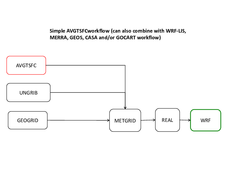
Regression Testing

Regression testing is a type of software testing that verifies that software previously developed and tested still performs correctly even after it was changed or interfaced with other software. Changes may include software enhancements, patches,configuration changes, etc. During regression testing, new software bugs or regressions may be uncovered.

Testing types

Software testing can be roughly divided into three categories:

Automated regression tests. These tests compile and run a very large number of model configurations and may perform various checks.
Manual/user testing. These tests are intended to be performed by users that wish to verify their changes prior to pushing them to a central repository. In detail, these tests are similar to automated tests, but are more easily executed from the command line.
Unit tests. These tests execute extremely quickly and provide a finer-grained verification than the other regression tests, albeit with far less coverage of the source code. Unit tests do not form part of the NU-WRF code base at this time.

In this section, we discuss the available NU-WRF regression testing infrastructure and how it can be used to perform automated and manual tests.

NU-WRF regression testing scripts

The NU-WRF regression scripts are a set of python scripts and
configuration files designed to run tests on the NU-WRF code base. The
scripts’ functionality is all driven by the settings specified in a
single configuration file.
The configuration file is a text file with a particular structure
readable by the python scripts and easily understood by humans too!
The files are organized into sections, and each section contains
name-value pairs for configuration data.
There is one configuration file required by the scripts - specified as
a command line argument. The file can have any name but must have the
’.cfg’ extension. A sample configuration file (sample.cfg) is included
in scripts/python/regression that can be modified and used for
“personalized” testing.
There are three additional files that are used specifically for NU-WRF
testing. Specifically master.cfg, develop.cfg and comp.cfg. These
files should not be modified or used for anything other than as a
reference to build your own customized configuration.

Workflows revisited

In this chapter, we discussed several workflows. For the purposes of regression testing workflows are categorized as follows:

wrf: basic WRF-ARW runs (without LIS coupling)
wrflis: wrf but with LIS coupling (including single-column model)
chem: wrf with chemistry (chemistry with or without LIS coupling)
kpp: wrf with chemistry using KPP

This distinction is necessary to specify test cases in the configuration file. For a list of all supported NU-WRF configurations see the file master.cfg under scripts/python/regression.

Python scripts

The python scripts are the following:

reg : Main driver.
RegPool.py : A class with functionality to parallelize tasks.
regression.py : A driver script to execute the NU-WRF component tasks.
RegRuns.py : A class that defines regression test run instances.
RegTest.py : A class that defines regression test instances.
reg_tools.py : Various tools used by the main drivers.
reg_utils.py : Various utilities used by all the scripts.

The scripts can be used to perform both automated regression tests as well as “manual testing”.

Manual testing

Before running the regression testing scripts make sure you duplicate the sample.cfg file and customize it to your needs. When ready to run the scripts, specify the configuration file name as an argument to reg and wait for the results:

$ cd $NUWRFDIR/scripts/python/regression

To run the scripts, specify the configuration file name as an argument to reg:

$ reg <cfg_file> &

Note that the configuration file name extension should not be specified. Upon execution you will see some messages echoed to STDOUT but all the output will be logged to a file named $<$ cfg_file $>$ .LOG. There will be other “log” files, one for each workflow and one for each experiment, that will be generated for each ’reg’ run.

Workflow builds, a maximum of four (wrf,wrflis,chem,kpp), will be generated in

<scratch_dir>/builds

Each build will have its own make.log as well as $<$ workflow $>$ .out and $<$ workflow $>$ .err files that will be useful to diagnose build /run errors.

Run logs will be generated in each run directory under $<$ scratch_dir $>$ /results. These will have the name $<$ experiment $>$ -regression.log and should also be very useful to diagnose test-case-specific run-time issues.

At the end of a “reg” an email test report will be emailed to the recipient specified in the mail_to field in USERCONFIG.

Note that all ’reg’ runs are tagged with a unique time stamp corresponding to the date/time the run was executed.

As you may have figured out, all the workflows described earlier in this chapter can be recreated with the appropriate configuration file and the testing scripts.

Finally, there are many testcases found in the testcases subdirectory containing script templates for end-to-end workflows that can be used as starting points for setting up NU-WRF simulations.

For more information about regression testing or any workflow described in this tutorial please feel free to contact the NU-WRF software integration group.

Post-Processors

In Front End Workflows, sample workflows are presented to initialize and run WRF in multiple configurations. In the present section, we address the question of post-processing the WRF (and in some cases, LIS) output. All of the post-processors address the task of evaluation, either subjective or objective. Several tools are available to prepare visualizations of model fields, while others allow for calculating verification metrics against observations or gridded analyses.

It should be noted that other generic tools exist that can be used to evaluate NU-WRF netCDF4 output. These include:

IDL (https://www.nv5geospatialsoftware.com/Products/IDL);
IDV (http://www.unidata.ucar.edu/software/idv/);
MATLAB (https://www.mathworks.com/products/matlab.html);
NCL (http://www.ncl.ucar.edu);
Ncview (https://cirrus.ucsd.edu/ncview/);
Python (http://www.python.org) with:
- Matplotlib (http://matplotlib.org) or;
- PyNGL and PyNIO (https://www.pyngl.ucar.edu);
R (http://www.r-project.org) with:
- ncdf4 (https://cran.r-project.org/web/packages/ncdf4/index.html); or
- RNetCDF (https://cran.r-project.org/web/packages/RNetCDF/index.html);
VAPOR (https://www.vapor.ucar.edu).

See also a list of netCDF-compatible software maintained at http://www.unidata.ucar.edu/software/netcdf/software.html.

G-SDSU

The Goddard Satellite Data Simulator Unit [G-SDSU; Matsui et al. (2014) is a program developed by NASA for use with cloud-resolving model data. The program can simulate multiple microwave, radar, visible and infrared, lidar, and broadband satellite products from the input model fields. These simulations can be used for detailed verification against actual satellite observations Matsui et al. (2009), for assimilation of satellite radiances, or for exploring future satellite missions. The software is compiled by typing ./build.sh gsdsu. Instructions on running the program are available in Matsui and Kemp (2016).

RIP4

The community Read/Interpolate/Plot (RIP) Version 4 software package is capable of processing WRF netCDF files, deriving new variables (e.g., air temperature, relative humidity, CAPE), interpolating to isobaric, isentropic, or constant height levels as well as vertical cross-sections, and plotting the fields in NCAR Graphics gmeta format. Advanced options also exist, including calculating and plotting trajectories, interpolating between coarse and fine grid resolutions, and writing data in a format readable by the Vis5D visualization package (see http://vis5d.sourceforge.net).

The RIP software is compiled by typing ./build.sh rip. The two most important executables in RIP4 are:

RIPDP_WRFARW. This program will read WRF netCDF files and transform the data to an internal binary data format. The user will have the option of processing either a basic set of variables or all the variables in the files.
RIP. This program will process the output of RIPDP_WRFARW based on the user’s settings in a provided input file.

Users are referred to Stoelinga (2006) for detailed instructions on using RIP. Sample namelist files are included in the NU-WRF package in scripts/rip/.

ARWPOST

The ARWPOST program is a post-processor developed by NCAR for converting WRF-ARW netCDF data into GrADS format. Analogous to RIP, ARWPOST supports the derivation of certain variables from the model output and interpolation of those fields to isobaric or constant height levels. GrADS (see http://cola.gmu.edu/grads/) can then be used to visualize the data. The program is compiled by typing ./build.sh arw. Instructions for running ARWPOST are given in Chapter 9 of NCAR (2022).

UPP

The UPP program is the “Unified Post-Processor” developed by NOAA/NCEP for processing all NCEP model data. As with RIP and ARWPOST, UPP can read WRF netCDF output files, derive a number of meteorological fields from the provided model data, and interpolate to user specified levels. In the case of UPP, the data are output in GRIB format. The program is compiled by typing ./build.sh upp. Instructions for running UPP are given in DTC (2015).

The NU-WRF version of UPP includes several modifications provided by NASA SPoRT. These are experimental severe weather diagnostics:

Instantaneous Lighting Threat 1. Based on grid-resolved graupel flux at -15C. Specified as “LIGHTNING THREAT 1” in parm/wrf_cntrl.parm file.
Instantaneous Lightning Threat 2. Based on vertically integrated ice. Specified as “LIGHTNING THREAT 2” in parm/wrf_cntrl.parm file.
Instantaneous Lightning Threat 3. Based on Threat 1 and 2 products. Specified as “LIGHTNING THREAT 3” in parm/wrf_cntrl.parm file.
Interval Maximum Lighting Threat 1. Based on grid-resolved graupel flux at -15C. Specified as “MAX LTG THREAT 1” in parm/wrf_cntrl.parm file.
Interval Maximum Lightning Threat 2. Based on vertically integrated ice. Specified as “MAX LTG THREAT 2” in parm/wrf_cntrl.parm file.
Interval Maximum Lightning Threat 3. Based on Threat 1 and 2 products. Specified as “MAX LGT THREAT 3” in parm/wrf_cntrl.parm file.

In addition, UPP has been modified to read both graupel and hail mixing ratios, which are provided by the 4ICE microphysics scheme. Since the NCEP GRIB2 table does not list “hail” as a variable, hail is added to graupel for output and for use in visibility or radiance calculations. Also, UPP will read in radar reflectivity from the WRF output (variable REFL_10CM) if the 3ICE or 4ICE microphysics scheme was used, and this field will be used for any requested reflectivity product (in contrast, UPP calculates reflectivity for other microphysics schemes).

MET

The MET software is a community meteorological verification toolkit developed by the DTC. This is a generic tool for comparing gridded model forecasts and analyses against numerous observations – METARs, Mesonets, rawinsondes, MODIS satellite data, and Air Force cloud analysis data. MET expects the model data to be in GRIB format, a requirement that forces the user to run UPP on the WRF output first (see UPP section above). Observation data formats include PREPBUFR and MADIS. With this input data, MET can be used for a number of different meteorological verifications, including point-to-point verification, object-oriented verification, and wavelet verification. Numerous statistical measures can be calculated with confidence intervals, and plotting capabilities are available.

The MET software is compiled by typing ./build.sh met. Thorough instructions on running the software are provided in DTC (2021).

LVT

LVT is a NASA-developed land surface verification toolkit. It is designed to compare LIS output files against numerous in-situ, remotely sensed, and reanalysis products. Fields that can be evaluated include surface fluxes, soil moisture, snow, and radiation. Multiple verification metrics can be calculated, and advanced features include data masking, time series, temporal averaging, and analysis of data assimilation impacts. The software is compiled by typing ./build.sh lvt. Detailed instructions on running LVT can be found in NASA (2022c).

Frequently Asked Questions

Q:

What modules should I use on Discover and Pleiades when running NU-WRF?

A:

Modules are automatically loaded if you used the build.sh script provided with NU-WRF. The current defaults on Discover are (assuming Bash shell):

LIBDIR_TAG=/discover/nobackup/projects/nu-wrf/libs/sles15/intel-intelmpi

umask 022
. /usr/share/modules/init/bash
module purge
unset LD_LIBRARY_PATH
module load comp/gcc/12.3.0
module load comp/intel/2021.4.0
module load mpi/impi/2021.4.0
module load python/GEOSpyD/Min23.5.2-0_py3.11

export LD_LIBRARY_PATH=$LIBDIR_TAG/zlib/lib:$LD_LIBRARY_PATH
export LD_LIBRARY_PATH=$LIBDIR_TAG/hdf5/lib:$LD_LIBRARY_PATH
export LD_LIBRARY_PATH=$LIBDIR_TAG/netcdf4/lib:$LD_LIBRARY_PATH
export LD_LIBRARY_PATH=$LIBDIR_TAG/esmf/lib:$LD_LIBRARY_PATH
export LD_LIBRARY_PATH=$LIBDIR_TAG/openjpeg/lib:$LD_LIBRARY_PATH
export LD_LIBRARY_PATH=$LIBDIR_TAG/jpeg/lib:$LD_LIBRARY_PATH
export LD_LIBRARY_PATH=$LIBDIR_TAG/jasper/lib:$LD_LIBRARY_PATH
export LD_LIBRARY_PATH=$LIBDIR_TAG/gdal/lib:$LD_LIBRARY_PATH
export LD_LIBRARY_PATH=$LIBDIR_TAG/fortrangis/lib:$LD_LIBRARY_PATH
export LD_LIBRARY_PATH=$LIBDIR_TAG/eccodes/lib:$LD_LIBRARY_PATH
export LD_LIBRARY_PATH=$LD_LIBRARY_PATH:/usr/lib64
export PATH=$LIBDIR_TAG/netcdf4/bin:$PATH

And on Pleiades:

LIBDIR_TAG=/nobackupp17/nuwrf/toss/ekman/intel-hpempt

umask 022
. /usr/share/modules/init/bash
module purge
unset LD_LIBRARY_PATH
module load gcc/9.3
module load comp-intel/2020.4.304
module load mpi-hpe/mpt
module load python3/3.9.12

export LD_LIBRARY_PATH=$LIBDIR_TAG/zlib/lib:$LD_LIBRARY_PATH
export LD_LIBRARY_PATH=$LIBDIR_TAG/hdf5/lib:$LD_LIBRARY_PATH
export LD_LIBRARY_PATH=$LIBDIR_TAG/netcdf4/lib:$LD_LIBRARY_PATH
export LD_LIBRARY_PATH=$LIBDIR_TAG/esmf/lib:$LD_LIBRARY_PATH
export LD_LIBRARY_PATH=$LIBDIR_TAG/openjpeg/lib:$LD_LIBRARY_PATH
export LD_LIBRARY_PATH=$LIBDIR_TAG/jpeg/lib:$LD_LIBRARY_PATH
export LD_LIBRARY_PATH=$LIBDIR_TAG/jasper/lib:$LD_LIBRARY_PATH
export LD_LIBRARY_PATH=$LIBDIR_TAG/gdal/lib:$LD_LIBRARY_PATH
export LD_LIBRARY_PATH=$LIBDIR_TAG/fortrangis/lib:$LD_LIBRARY_PATH
export LD_LIBRARY_PATH=$LIBDIR_TAG/eccodes/lib:$LD_LIBRARY_PATH
export LD_LIBRARY_PATH=$LD_LIBRARY_PATH:/usr/lib64
export PATH=$LIBDIR_TAG/netcdf4/bin:$PATH

If you must change the modules (perhaps to test a different compiler version) or port to a new platform make sure that you modify the settings in scripts/other/set_module_env.bash. This includes specifying the location of third-party libraries used by NU-WRF.

The module settings should be done in your shell if you are running a program at the command line. If instead you are launching a batch job to SLURM or PBS, the above settings should be in the batch script, so the commands are run on the allocated compute node.

Q:

What other environment settings should I use?

A:

Make sure to set stack size to unlimited. This can help prevent memory allocation errors for automatic arrays. If using bash:

ulimit -s unlimited

If using csh:

limit stacksize unlimited

Q:

What namelist settings should I use with WRF?

A:

It is not possible to provide a single configuration optimal for all types of simulations (LES, regional climate, cloud system resolving, chemical transport, etc), but the settings in the testcases directory that provide several starting points. Each test case contains a README file that summarizes the experiment. Additionally, the table below shows a good first guess:

Porting NU-WRF

Currently NU-WRF is only fully supported for Intel compilers, for SGI MPT (on Discover and Pleiades), and for Intel MPI (on Discover). The current development branch also works with GNU compilers and OpenMPI or MVAPICH2 on Discover. The underlying software should, however, run on other systems as long as the appropriate tools (compilers, MPI implementation, make, Perl, csh, bash, etc.) are available. Users who wish to port NU-WRF will need to take the following steps:

Libraries:
- Compile the libraries listed in the External Libraries and Tools section.
- Determine the paths to the yacc binary and the flex library. Make sure yacc and flex are in your PATH environment variable.
- Copy scripts/python/build/nu-wrf.cfg to a new top level build configuration file (here called newconfig.cfg, but any unique name can be used).
- Edit newconfig.cfg and update the library paths.
- Edit scripts/other/set_module_env.bash. Remove hardwired checks for pleiades and discover that will abort execution of the script. Next, set LIBDIR_TAG and change modules for system binaries and libraries (compilers, MPI, etc). If the Environmental Modules package (http://modules.sourceforge.net/) is not installed on your system, comment out the module commands and explicitly edit the PATH and LD_LIBRARY_PATH environment variables.
ARWPOST:
- Inspect and edit ARWpost/arch/configure.defaults to ensure a block exists for the desired operating system, hardware, and compilers. Note that ARWPOST is serial only (no MPI support).
- Run ARWpost/configure at the command line to identify the integer value of the appropriate build selection.
- Edit newconfig.cfg to enter the configure option as environment variable ARWPOST_CONFIGURE_OPT.
- In the top NU-WRF directory, run ./build.sh --config newconfig.cfg arwpost to test the build.
GSDSU:
- Create a new makefile template in directory postproc/GSDSU/SRC/ specifying the appropriate compilers, compiler flags, and MPI library if applicable.
- Edit newconfig.cfg to enter the new makefile template name as environment variable GSDSU_MAKEFILE.
- In the top NU-WRF directory, run ./build.sh --config newconfig.cfg gsdsu to test the build.
LDT:
- Edit LISF/ldt/arch/Config.pl to specify the compiler flags. Compilers are specified using the LDT_ARCH environment flag (e.g., ‘linux_ifc’ indicates Intel compilers on Linux).
- Edit newconfig.cfg to specify the correct LDT_ARCH value. If necessary, also edit the LDT_FC and LDT_CC variables to specify the correct MPI compiler wrappers.
- In the top NU-WRF directory, run ./build.sh --config newconfig.cfg ldt to test the build.
LVT:
- Edit LISF/lvt/arch/Config.pl to specify the compiler flags. Compilers are specified using the LVT_ARCH environment flag (e.g., ’linux_ifc’ indicates Intel compilers on Linux).
- Edit newconfig.cfg to specify the correct LVT_ARCH value. If necessary, also edit the LVT_FC and LVT_CC variables to specify the correct MPI compiler wrappers.
- In the top NU-WRF directory, run ./build.sh --config newconfig.cfg ldt to test the build.
MET:
- Edit newconfig.cfg to set the CXX, CC, and F77 environment variables, which defines the names of the C++, C, and Fortran compilers, respectively.
- In the top NU-WRF directory, run ./build.sh --config newconfig.cfg met to test the build.
RIP4:
- Inspect and edit RIP4/arch/configure.defaults to ensure a block exists for the desired operating system, hardware, and compilers. Note that RIP4 is serial only (no MPI support).
- Run RIP4/configure at the command line to identify the integer value of the appropriate build selection.
- Edit newconfig.cfg to enter the configure option as environmental variable RIP_CONFIGURE_OPT.
- In the top NU-WRF directory, run ./build.sh --config newconfig.cfg rip to test the build.
UPP:
- NOTE: Make sure WRF is ported first.
- Inspect and edit UPP/arch/configure.defaults to ensure a block exists for the desired operating system, hardware, compilers, and MPI implementation.
- Run UPP/configure at the command line to identify the integer value of the appropriate build selections.
- Edit newconfig.cfg to enter the configure option as environment variable UPP_CONFIGURE_MPI_OPT.
- In the top NU-WRF directory, run ./build.sh --config newconfig.cfg upp to test the build.
WPS:
- NOTE: Make sure WRF is ported first.
- Inspect and edit WPS/arch/configure.defaults to ensure a block exists for the desired operating system, hardware, compilers, and MPI implementation.
- Run WPS/configure at the command line to identify the integer value of the appropriate build selection.
- Edit newconfig.cfg to enter the configure option as environmental variable WPS_CONFIGURE_MPI_OPT. If necessary, also edit the WPS_DEBUG_CFLAGS, WPS_DEBUG_FFLAGS, and WPS_DEBUG_F77FLAGS variables to specify appropriate debugging flags for your compilers.
- In the top NU-WRF directory, run ./build.sh --config newconfig.cfg wps to test the build.
WRF and LIS:
- Inspect and edit WRF/arch/configure_new.defaults to ensure a block exists for the desired operating system, hardware, compilers, and MPI implementation.
- Run WRF/configure to identify the integer value of the appropriate build selection.
- Create a new configure.lis makefile template in LISF/lis/arch/ with appropriate compiler selection. NOTE: This approach is used instead of running the LIS configure script because LDFLAGS must be absent from the configure.lis file if the LIS code is compiled for coupling; also, it is easier to pass consistent debugging compiler flags to WRF and LIS by having the NU-WRF build system do it on the fly.
- Edit the newconfig.cfg to enter the configure option as environmental variable WRF_CONFIGURE_MPI_OPT. Also list the makefile template with environmental variable WRF_CONFIGURE_LIS_MPI. Also, set environmental variable LIS_ARCH to the value appropriate for your operating system and compiler [see (NASA 2022b) for options]. If necessary, also edit the WRF_DEBUG_CFLAGS_LOCAL and WRF_DEBUG_FCOPTIM variables to specify appropriate debugging flags for your compilers.
- In the top NU-WRF directory, run ./build.sh --config newconfig.cfg wrf to test the build. Also test with the chem and kpp targets.

Porting the programs under utils/ (GEOS2WRF, CASA2WRF, SST2WRF, etc.) only requires that the file path of the external NU-WRF libraries, LIBDIR_TAG, described at the end of section 4.4 be correctly specified.

Revision History

For updated information see https://nuwrf.gsfc.nasa.gov/whats-new.

Version 9 Patch 3 (v9p3-wrf391-lis72; “Charney Patch 3”).
- Added support for WRF-NoahMP-3.6 coupling
  - Test cases
    - noah36_modis_gdas_lis_spinup
    - noahmp_modis_gdas_lis_spinup
    - noahmp_modis_merra2_lis_spinup
- WRF Physics
  - DOE CRM
    - utilizes WRF as a CRM/LES using doubly periodic lateral boundaries
  - NTU (National Taiwan University) microphysics
    - A multi-moment four-ice (pristine ice, aggregate, graupel, and hail) bulk microphysical scheme
  - WRF electrification scheme
- Upgraded Intel compiler version to 18.x, consistent with LISF.
- NEVS: Updated documentation and organization to make it easier to use
Version 9 Patch 2 (v9p2-wrf391-lis72; “Charney Patch 2”). This is a bug fix patch.
- Fixed a problem observed in LIS precipitation being consistently less than that coming from WRF and which was due to a unit conversion issue. This bug may impact some results, specifically soil moisture and overall soils wet/dryness, for very long simulations.
- This release also contains several build system enhancements that had already been merged into the develop branch.
Version 9 Patch 1 (v9p1-wrf391-lis72; “Charney Patch 1”)
- Corrections to WRF 3.9.1 merge (on the recommendation of NCAR core team).
  - Move some initializations to physics init to avoid race conditions.
  - Remove file remnants from WRF 3.7.1.
  - Renamed NU-WRF diagnostics modules to conform with WRF conventions.
- Replaced bash-based build mechanism with a python-based one (see Section 4.3).
  - Standardized interface to differentiate between required and optional arguments.
  - Standardized build steps (clean, configure, build, install).
- Updated regression testing suites.
  - Corrections to various tests.
  - Added standard ARW tests.
  - Added WRF-Lake tests.
  - Added tests that perform a LIS spinup.
  - Added support for Pleiades testing.
- Upgraded Intel compiler version to 17.0.4.196.
- Upgraded GNU compiler version to 6.3.
- Updated NU-WRF User Guide.
- Updated tutorial documentation and testcases.
- Note on MET component: New compilers are incompatible with MET 6.x, so we have made a temporary revert to v5.1.
Version 9 (v9-wrf391-lis72; “Charney”)
- Upgraded to WRF 3.9.1.
  - Added 2017 Goddard radiation scheme. (uses one LUT: BROADBAND_CLOUD_GODDARD.nc)
  - New longwave and shortwave radiation options are ra_lw_physics=57 and ra_sw_physics=57 respectively.
  - Updated Registry.EM_COMMON and Makefile accordingly.
- Upgraded to WRF-chem 3.9.1.
- Upgraded to WPS 3.9.1.
  - Update GEOGRID.TBL.ARW table.
- Upgraded to MET 6.0.
- Upgraded to UPP 3.1.1.
- Applied RIP4 2017 updates.
- Upgraded Intel compiler version to 17.0.1.132.
- Updated NU-WRF User Guide.
- Updated regression testing suites.
  - Removed 2011 Goddard radiation scheme tests.
  - Removed Noah 2.7.1 and Noah 3.2 tests.
  - Added 2017 Goddard radiation scheme tests.
  - Updated GFEDv3 tests to use GFEDv4 option.
  - Added new option to setup run scripts.
  - SOILPARM table in lis.config is now read from noah3X_parms directory.
Version 8 Patch 5 (v8p5-wrf371-lis72r; “Bjerknes Patch 5”)
- Ported under GNU.
  - Ported utils and fixed issues with parallel compilation.
  - There are some tweaks in RIP4, LDT, LVT, WPS and WRFV3.
- Added scripts to facilitate installation of third-party libraries and to help with code porting (see scripts/other/baselibs.*) .
- Significant refactoring of regression testing scripts that include
  - Fixing commands that trigger nonzero return code.
  - Adding a new file, check_nuwrf_repo.py, to monitor, via cron, the new git repo.
  - Adding a new script,diffnc4.py, to compare netcdf4 files produced by WRF.
- Consolidated discover/pleiades cfg scripts into one (nu-wrf.cfg).
- Moved build_ldt and build_lvt into respective directories and simplified top level build.sh accordingly.
- Add install option when running build.sh.
  - If environment variable NUWRF_INSTALL_DIR is defined then all executables will be installed in that directory.
- Upgraded LVT/LDT/LIS to version 7.2r.
  - Add user.cfg to temporarily disable RUC. When RUC option is set to True, various subroutine stubs in RUC conflict with duplicate ones in WRF. As a result, the RUC option has been temporarily disabled.
  - LVT failed to compiled due to an assumption in file readGIMMSMODIS_NDVIObs.F90 where GDAL use was always expected. File was modified for NU-WRF and the assumption was removed.
- Added functionality to prep_chem_sources to deal with GFEDv4 sources.
  - The utils code required additional code to process GFEDv4 data, specifically a module to read HDF5 files and a tokenizer for string conversion.
- Added scripts that make up the NU-WRF Ensemble Verification System
- LIS workaround to deal with input files that contain no land points.
- Updated user guide and tutorial.
Version 8 Patch 4 (v8p4-wrf371-lis71rp8; “Bjerknes Patch 4”)
- Added new NU-WRF regression testing scripts and configurations in scripts/regression directory.
- Updated CASA2WRF pre-processor allowing a moving average window option for smoothing daily $C O_{2}$ flux data.
- Upgraded LDT to version 7.1rp3. Also updated LDT 7.1 User Guide in docs/ directory to version released in November 2016.
- Upgraded LIS to version 7.1rp8, plus additional patch in MERRA2 metforcing to support lapse-rate correction option.
- Added NU-WRF tutorial material in docs/ directory.
- Added new ideal_scm_lis_xy build target. Compiles WRF IDEAL preprocessor to produce inputs for running coupled WRF-LIS in idealized Single Column Mode.
- Added build support for community WRF ideal_b_wave, ideal_convrad, ideal_heldsuarez, ideal_les, ideal_quarter_ss, ideal_scm_xy, and ideal_tropical_cyclone data cases. (Other idealized cases will not compile at this time.)
- Added LIS4SCM preprocessor to make LDT and LIS output files horizontally homogeneous for use in NU-WRF WRF-LIS Single Column Mode.
- Added scripts for created Single Column Mode forcing from METGRID output (borrowed from Josh Hacker, NCAR).
- Updated 4ICE microphysics hand-vectorized by Jarno Mielikainen (University of Wisconsin), plus a bug fix for calculating hail intercept parameter.
- Updated 2014 radiation scheme hand-vectorized by Jarno Mielikainen (University of Wisconsin).
- Refactored NU-WRF utils to consolidate code and simplify build mechanism.
- Added new ./build.sh utils target to compile all utils/ programs.
- Moved User Guide LaTeX files to docs/ directory.
- Remove -ip Intel compiler flag at suggestion of NCAR.
Version 8 Patch 3 (v8p3-wrf371-lis71rp7; “Bjerknes Patch 3”)
- Added support for ECMWF T511 Nature Run files:
  - UNGRIB now supports N256 Reduced Gaussian Grid GRIB files.
  - Added Vtable files for N256 data.
  - Added ecmwf_coeffs_L91 file listing hybrid sigma-pressure coefficients.
  - Added script for CALC_ECMWF_P preprocessor.
- LDT bug fix for compiler warning in ldt/metforcing/cmorph.F90 about external function not given explicit type.
- LIS bug fixes:
  - Fixes for warning in
    
    WRFV3/lis/surfacemodels/land/clm2/csm_share/clm2_shr_sys_mod.F90 about unused argument (related to use of preprocessor flags).
  - Fix for warning in WRFV3/lis/surfacemodels/land/mosaic/umd_sibalb.F90 about function not given an explicit type.
Version 8 Patch 2 (v8p2-wrf371-lis71rp7; “Bjerknes Patch 2”)
- Critical patch. Added LIS irrigation support to WRF-LIS coupling. This was overlooked in earlier versions of Bjerknes.
- Modified LIS to change default output directory permissions to a+rwx. This can be further restricted at run-time by the umask shell command.
Version 8 Patch 1 (v8p1-wrf371-lis71rp7; “Bjerknes Patch 1”)
- Critical patch. Changed REAL to always copy TSK and TMN from the grid data structure tsk_gc and tmn_gc members before merging LIS data. This corrects a fatal error when processing METGRID and LIS data without a separate sea surface temperature field.
- Critical patch. Added TLAG variable to WRF restart file (via Registry.EM_COMMON). This patch was released by NCAR on 8 Sep 2016 to fix a problem with dynamic deep soil temperature in WRF 3.7, 3.7.1, 3.8, and 3.8.1.
- Updated external libraries:
  - New libraries. Added GDAL 2.1.1 and FORTRANGIS 2.5. These are used by the new NDVIBARENESS4WRF utility.
  - Upgraded to ESMF 6.3.0rp1, FREETYPE 2.6.5, G2CLIB 1.6.0, GRIB_API 1.17.0, GSL 2.2.1, HDF4 4.2.12, HDF5 1.8.17, NETCDF 4.4.1, NETCDF-Fortran 4.4.4, and PIXMAN 0.34.0.
  - NUWRFLIB library package on Discover and Pleiades upgraded to version 8r2.
- UPP patches:
  - Now reads REFL_10CM variable from WRF netCDF output when processing radar reflectivity from 3ICE or 4ICE microphysics scheme, instead of searching for non-existent DBZ variable.
  - Removed redundant deallocation statements for lightning product, which were causing UPP to crash.
- Added NDVIBARENESS4WRF utility, which can process GIMMS or SPoRT MODIS NDVI products and create a “bareness” field for dynamic dust emissions.
- Added fetch_sport_sst_northwestHemi.py script to download real-time SPoRT SST GRIB2 files. Script and configuration file are in the new scripts/fetch_data/ directory.
- Updated UNGRIB to set all negative SST values to -1.E30 (the default missing flag used by METGRID). This allows processing the SPoRT SST product without changing the default missing flag.
- LISCONFIG patches:
  - Map projection now output by Fortran program LISWRFDOMAIN for insertion into ldt.config file.
  - lisWrfDomain.py now checks to see if any domain settings returned by the Fortran program are unused when updating ldt.config and lis.config. This is assumed to indicate an error with the input file templates (i.e., a configuration setting is missing in the template), which can easily happen if the template is for a different map projection when what WRF will use.
- Added initialization of dx and dy variables in METGRID when processing cylindrical equidistant (lat-lon) or Gaussian data. This fixes an interpolation problem.
- Changed WPS INT2NC utility to output data in netCDF4.
- Minor bug fixes to sample batch configuration files.
Version 8 (v8-wrf371-lis71rp7; Official “Bjerknes” Release)
- Merged WRF 3.7.1, WPS 3.7.1, PREP_CHEM_SOURCES 1.5, RIP 4.6.7, UPP 3, and MET 5.1, plus community patches released through May 2016.
- Merged LIS 7.1rp7 and LDT 7.1rp2, including fixes for Mercator map projection.
- Upgraded Intel compilers to 15.0.3.187. Default MPI implementation on both Discover and Pleiades is SGI MPT. Intel MPI 5.1.2.150 is also suppported on Discover (for legacy Sandy Bridge nodes). GFORTRAN 4.9.0 and OpenMPI 1.7.3 are temporarily supported for debugging (specifically with VALGRIND). Retired Intel MPI 4 support on Pleiades.
- Removed -xSSE4.2 hardware specific Intel compiler flag. Tests show no consistent performance improvement.
- Modified build system to require MPI for WRF, WPS, and UPP (no serial builds permitted).
- External libraries are now packaged in separate NUWRFLIB collection. This NU-WRF release links against NUWRFLIB 8r1 on Discover and Pleiades. This includes new dependencies (CAIRO, FREETYPE, GHOSTSCRIPT, and PIXMAN) and updates to older dependencies.
- Added sample namelist, lis.config, and ldt.config files for multiple test cases. The LIS cases include use of SRTM 30 sec topography and “slope-aspect” correction which improves the spin-up of soil moisture.
- Updated SST2WRF processing: Changed output mask to separately indicate “low confidence” and “high confidence” SST points. “Low confidence” SST data are now included in output (originally were flagged as bad, but this has a high false alarm rate in the C3VP test case).
- Updated METGRID processing: SST is now interpolated with parabolic, bi-linear, weighted 4-pt average, or weighted 16-pt average (tried in order until one works). When processing TAVGSFC (from AVG_TSFC preprocessor), METGRID tries parabolic before bi-linear interpolation. This helps reduce data voids and discontinuities in (blended) SST field.
- Updated REAL processing:
  - Preserves LIS greenness and albedo data but processes time-varying LAI data from GEOGRID and METGRID.
  - Changed SST processing to check for obviously bad ocean SSTs when 30s MODIS+Lakes land data are used. Also, disabled use of TAVGSFC as a replacement for bad ocean SST (it seems better to just use skin temperature in this case).
- Added option to skip compiling of WRF CLM4 code. CLM4 is not used by GSFC, and this saves about 10 minutes of build time.
- WRFV3 files module_first_rk_step_part1.F and module_comm_dm_4.f90 are now on the “do not optimize” list to cut down on build times (saves about 10 minutes).
- Multiple bug fixes to prevent memory corruption with arrays allocated with size 1 instead of with WRF “memory” dimensions.
- Updated GEOGRID.TBL files to make GEOGRID.TBL.ARW_CHEM_NUWRF a strict superset of GEOGRID.TBL.ARW_CHEM, with the latter now a strict superset of GEOGRID.TBL.ARW.
- Updated dynamic dust emissions. The temperature of the second soil layer is now used instead of skin temperature to detect frozen soil and shut off emissions (this fixes a diurnal cycle bias). Also, the threshold for snow depth is raised to 0.01 m (was zero).
- Increased geopotential height threshold to discriminate between oceans and lakes in sea salt emission calculation.
- Connected the GOCART sulfate chemistry with the RADM2 gas phase chemistry to account for the heterogeneous conversion of SO $_{2}$ to sulfate. Previously such conversion was not sufficiently represented in RADM2.
- Redistribution of BC and OC emissions into BC1, BC2, OC1, OC2 aerosol species. This way the NU-WRF aerosol algorithm will be in line with the global GOCART version.
- Added handling of both cumulative diabatic heating (K) and “snapshot” diabatic heating rates (K/s) from 3ICE and 4ICE microphysics schemes. Cumulative heating is now written to restart file.
- 4ICE microphysics updates:
  - Change to “melting” diabatic heating rate to account for wet hail accretion.
  - Adjusted intercept scaling factors are now used to calculate reflectivity.
- 3ICE microphysics update: Bug fix for warm rain code.
- Upgraded GSDSU to version 3.5.1. Changes include:
  - Add support for Thompson microphysics scheme.
  - Visible-IR simulator is more stable (less run-time crashes).
  - New statistical model for CRM diagnosis.
  - Updated GSDSU User Guide.
- CASA2WRF updated to add bug fixes for the following:
  - CO $_{2}$ flux output files now has CO $_{2}$ flux for time $t$ and flux tendency between time $t$ and time $t + 1$ .
  - Ocean CO $_{2}$ and fossil fuel data is on the corner of the grid instead of the middle point of the grid. All other components are at the midpoint of the grid.
- Added symbolic link to GODDARDRAD_SSLUT in WRFV3/run/ directory.
- Added fetch_rss_sst.sh script to download RSS SST data (more fault tolerant than Run_SST.csh),
- Added batch scripts to run WPS utility program AVG_TSFC.
- Updated Discover SLURM batch scripts to remove reference to sp1 constraint (no longer exists).
- Multiple bug fixes to initialize variables.
Version 7-3.5.1-p7 (Official “Arthur” Patch Release 7)
- Upgrades to LIS 7.1rp5, LDT 7.1rp1, and LVT 7.1rp1. Key changes include:
  - Updates to MERRA2 and MERRA-Land met forcing readers to work with certain LIS time step lengths. Also updates start and end dates for some MERRA2 streams.
  - Corrections to GDAS T170 domain and terrain data.
  - Updates to NLDAS-2 met forcing reader (improves rainfall and convective rainfall around island/coastal areas when downscaled to higher resolutions.)
  - Fix to pcp met forcing field when also reading snow.
  - Updated user guides.
- Added taucldc and taucldi to Goddard and CAM radiation package listings in Registry.EM_COMMON. These arrays are expected by the radiation schemes to be allocated with the WRF “memory” bounds, but WRF was allocating them with shape (1,1,1) instead. This caused memory corruptions.
- NUWRF 3ICE and 4ICE microphysics now output reflectivity as REFL_10CM.
- Removed DBZ array from grid data structure to save space. Updated sample RIP template sfcDBZUV.in to use REFL_10CM instead.
- COMDBZ now calculated in microphysics driver for every microphysics scheme where REFL_10CM is available.
- Updated Run_MERRA2.csh to use new path for MERRA2 data on Discover.
- Updated proc_merra2_ges_disc.sh to use new filename for MERRA2 terrain file on GES DISC web page.
- Retired old build configuration files for SLES 11 SP1 nodes on Discover (these no longer exist). Also removed obsolete DISCOVER_INSTRUCTIONS.TXT.
Version 7-3.5.1-p6 (Official “Arthur” Patch Release 6)
- Enabled WRF-LIS coupling for Noah 2.7.1, Noah 3.2, and Noah 3.6.
- WRF now passes pure LWDOWN (downward longwave radiation) to LIS without first multiplying by surface emissivity.
- Changed LIS Noah 2.7.1 to multiply LWDOWN by surface emissivity (already done in newer Noah versions).
- LIS exported surface emissivity now copied back to WRF array for input to radiation.
- Added capability for CASA2WRF to temporally interpolate the CO $_{2}$ flux depending on the NU-WRF state. CASA2WRF can now:
  - Read component CO $_{2}$ fluxes and interpolate to WRF grid.
  - Read WRF output.
  - Interpolate the CO $_{2}$ flux components based on shortwave radiation and surface temperature from WRF state, compute the net production of CO $_{2}$ , and compute the total flux and tendency.
  - Create input flux files from WRF-Chem runs with CASA CO $_{2}$ .
Version 7-3.5.1-p5 (Official “Arthur” Patch Release 5)
- Updated 4ICE microphysics scheme, and added aerosol coupling.
- Revised wrfout variable list to reduce file size and write times. Also added total latent heat rate calculation, and now passes dx to 4ICE scheme.
- Added MPI-safe convective-stratiform index diagnostic.
- Fixed asynchronous I/O (“quilting”) for coupled WRF-LIS.
- Changed REAL to use less memory when reading from LDT/LIS netCDF file.
- LIS updates:
  - Combined lisconfig_offline, lisconfig_coupled1, and lisconfig_coupled2 routines into lisconfig_generic.
  - Added VIIRS and SPoRT GVF testcases.
  - Added support to diagnose greenness in units of percentage.
  - Updated ldt.config files for the wrfout testcase.
  - Added nest loop to metForcGen_interp_finalize routine.
- GOCART2WRF updated to support MERRA-2 GOCART and offline GOCART data.
- Added proc_merra2_gocart_ges_disc.sh script to download MERRA-2 GOCART data from NASA GES DISC web page and process with GOCART2WRF.
- Added proc_merra2_ges_disc.sh script to download MERRA-2 meteorological data and process with MERRA2WRF.
- Disabled call to WRF-Chem optical driver when using 2011 or 2014 Goddard radiation.
- Bug fixes to GOCART volumetric mean refractive index calculation: (1) Removed erroneous copying of dust to “other inorganics”, which created spurious extra source of aerosols; and (2) removed MSA from refractive index calculation.
- Updated 2014 Goddard Radiation scheme:
  - Rescaled molecular absorption up 50% in shortwave scheme to correct severe underestimation of clear-sky atmospheric absorption. Value adjusted towards RRTMG scheme.
  - Increased CO $_{2}$ concentration.
  - New lookup tables for 4ICE microphysics.
  - Code changes to support OpenMP.
- Lateral boundary condition bug fix (cherrypicked from WRF 3.7).
- Increase in maximum I/O time levels.
- Added kinetic energy spectra scripts (from NASA DSCALE project).
- Upgraded GSDSU to version 3.5:
  - New global IR emissivity database from University of Wisconsin (Seemann et al. 2008).
  - Modified size boundaries for precipitating and non-precipitating particles (200- $μ$ m diameter threshold) for computing microwave/ visible/IR optical properties.
  - UV-VIS-IR non-spherical ice scattering database for VISIR simulator from Texas A&M University team (Yang et al. 2013).
  - Bug fixes for memory allocation, writing to netCDF output file, and handing MPI aborts.
  - Updated GSDSU User Guide.
- Modified LDT to output netCDF4 file for REAL if selected at compile time. Earlier code was hardwired to use classic netCDF3, which made LDT unusable for very large domains (e.g., $5000 \times 5000$ ).
- Bug fix to G3 cumulus scheme to prevent division by zero in Himalayas.
- Changed PREP_CHEM_SOURCES to support new 72-level GOCART background data files for actual year and month being processed. The user should edit prep_chem_sources.inp and set gocart_bg_data_type=“new”; create a gocart_bg_new/ subdirectory on the same level as the gocart_bg/ folder containing the community 55-level files; and store new
  
  geos5_met_1MAVG_YYYYMM.nc and gmi_merra_oxidants_YYYYMM_1.25x1.nc files in gocart_bg_new, where YYYY is the 4-digit year and MM is the 2-digit month. If PREP_CHEM_SOURCES cannot find both files, it will fall back on gmi_2006MM.nc files in gocart_bg_new/, which are also 72-levels but only exist for 2006.
- Added limited support in UPP for Goddard microphysics schemes. Graupel and hail mixing ratios are now read in. If the NU-WRF 3ICE or 4ICE scheme was used (instead of the community WRF version), then the DBZ field will also be read in. Radiance generation is disabled (use GSDSU for that). Since hail is not in the NCEP GRIB table, hail and graupel mixing ratios are combined. This may lead to problems with the GSD visibility product, but the proper extinction coefficients for hail are unknown.
Version 7-3.5.1-p4 (Official “Arthur” Patch Release 4)
- Upgraded LIS to 7.1r. This includes:
  - Noah 3.6, NoahMP 3.6, and CABLE 1.4b LSMs (only Noah 3.6 tested with NU-WRF).
  - Flood and drip irrigation.
  - VIIRS Daily GVF data
  - TRMM 3B42 V7 real time precipitation
  - Gaussian T1534 GFS met forcing data
  - MERRA-2 met forcing data (data only available to select users).
  - Downscaling precipitation (PRISM) (NLDAS-2 only)
  - Should compile now with gfortran.
- Upgraded LDT to 7.1r. Updates include:
  - Fixes to several metforcing readers that process the forcing terrain-height or elevation fields when processing model parameters.
  - Corrected conserved (budget-bilinear) interp routines. Users may notice slight differences in results.
  - MetTimeDScale and Metforcproc runmodes.
  - Crop, CLM2, Flake, Mosaic, Noah, SiB2, and VIC parameters.
  - TRMM 3B42 V7 real time precipitation.
  - Aquarius L2, GCOMW AMSR2 L3, and SMOS L2 soil moisture observations.
  - Simulated GRACE products.
- Upgraded LVT to 7.1r. Updates include:
  - Fixed bug affecting output of summary and final metric files.
  - GCOMW, ASCAT, SMOS, and SMOS L1 Tb observations.
  - MODIS LST and Great Lakes Hydro data.
  - Time lagged computations.
- Upgraded compiler version to Intel 13.1.3.192.
Version 7-3.5.1-p3 (Official “Arthur” Bug Fix Release 3)
- Updated pleiades.cfg to use new generic SGI MPT module on Pleiades. Older versions of SGI MPT are scheduled for removal on 6 July 2015, and users are advised to switch to the generic module to prevent future breakage when SGI MPT is upgraded and older versions are removed.
- Fixed netCDF4 chunking and deflation (compression) in GOCART2WRF when writing new chemistry fields to wrfinput and wrfbdy. Also removed unused variables from source code, and reorganized Makefiles.
- Added new temporalInterpolation GEOS2WRF tool, plus
  
  run_temporalInterpolation_merra2_3hr.discover.sh script to automate and interpolate 6-hourly MERRA-2 reanalyses to 3-hourly.
- Upgraded LIS to 7.0rp3.
- Added options to suppress dynamic dust emission and to spread dust across multiple near-surface levels.
- Updated sample batch scripts to check if SGI MPT, Intel MPI, or MVAPICH2 is used and invoke the corresponding appropriate run command when starting a MPI program (mpirun, mpiexec, mpiexec_mpt, or mpiexec.hydra).
- Modified ARWPOST to read wrfout files from WRF-Chem.
- Modified PREP_CHEM_SOURCES to support NASA QFED fire emissions.
- Modified Run_MERRA2.csh to allow user to override base path of MERRA-2 data via environment variable.
- Added build system option to compile WRF with Allinea MAP profiling libraries (only works on Discover).
Version 7-3.5.1-p2 (Official “Arthur” Bug Fix Release 2)
- Fixed WRF-Chem GOCART cloud fraction code to run when not using Grell cumulus scheme.
- Updates to LIS MERRA-Land reader code – better handling of missing input.
- Updated Run_MERRA2.csh script to reflect current stream status and to use consistent indentation.
- Added MERRA-2 support in LIS.
- Added run_geos2wrf_merra2_assim.discover.sh script to run GEOS2WRF to process 3-hourly MERRA-2 assimilation data (GEOS-5 output as the model is adjusting towards the MERRA-2 6-hr analyses via IAU). The collection for this data is a bit different than the 6-hr analyses, and it was easier to use GEOS2WRF rather than edit MERRA2WRF. Script only works on Discover, and assumes the user has access to the MERRA-2 GMAO directory on Discover.
- Added bug fix to GEOS2WPS to handle 3-hourly MERRA-2 assimilation data.
- Bug fix for MERRA-Land in LIS (fixes downward shortwave radiation index).
- Allow WRF to run with Noah LSM selection if REAL processed LIS data. Allows user to switch from WRF-LIS coupling to WRF-Noah-initialized-from-LIS without rerunning LIS to produce GRIB files.
- Updated LIS/LDT/LVT Makefiles to reduce number of include directories to search through (cuts down on build time).
- Fixed loops in WRF-Chem convective transport code to skip nv=1 (which is not a valid chemical species), and to loop through all chemical species instead of just gas (back ported from WRF-Chem 3.6.1).
- Added value for variable DELZ_THRESOLD in WRF-Chem plume model. Plume model with stop when plume top changes less than 100 meters over ten minutes.
- Bug fix to PREP_CHEM_SOURCES, resolving conflicting symbols imported from two different modules.
Version 7-3.5.1-p1 (Official “Arthur” Bug Fix Release)
- Modified build configuration files for Discover to check operating system version on computer used for compilation. New default configuration requires SLES 11.3 (same as the new Haswell nodes) and Intel MPI 5. A separate configuration file discover_intel13_sgimpt_sp3.cfg is also added to allow use of SGI MPT. Older Intel MPI 4 and MVAPICH2 configurations are moved to discover_intel13_impi4_sp1.cfg and discover_intel13_mvapich2_sp1.cfg, respectively, and require the older SLES 11.1 operating system.
- Fixed build configuration file pleiades_intel13_impi.cfg to compile on Pleiades with Intel MPI (default configuration uses SGI MPT).
- Merged in LIS 7.0rp2. Bug fixes: Do not reset Zh and Zm for processes with zero tiles; several VIC LSM related changes, and updates for CMAP.
- Merged in LDT 7.0rp2. Bug fixes to mapping between LIS fine Lambert Conformal grid and coarser Lat-Lon parameter grid extents. Also fixes domain extent checks for NLDAS-1 and NLDAS-2 forcing.
- Bug fixes to Goddard 2011 and 2014 radiation schemes. Transmission functions in the CO2, O3, and three water vapor bands with strong absorption are now computed using table look-up. Significantly improves accuracy for pressures less than 10 mb.
- Modified WRF and LIS configure templates to add -xCORE-AVX2 compiler flag options. However, early tests show slower run times compared to -xSSE4.2, so the build configuration files do not currently use them.
- Merged in Weile Wang’s (NASA ARC) modifications to the WRF spectral nudging code. FFT runs significantly faster with Weile’s changes.
- Modified WRF code to fix -DBENCH instrumentation for most parts of the WRF solver.
- Added Python scripts to calculate summary metrics from WRF RSL files for benchmarking.
- Modified MERRA2WRF to add preliminary support for MERRA-2 data files released to select users by the GMAO. “Official” support will not occur until after MERRA-2 is released to the general public.
- Build system fixes for handling CASA preprocessors.
- Updated sample Discover batch scripts for Haswell nodes.
Version 7-3.5.1 “Arthur” (Official Release)
- Merged WRF 3.5.1, WPS 3.5.1, PREP_CHEM_SOURCES 1.3.2, RIP 4.6.5, UPP 2.1, and MET 4.1.
- Merged LIS 7.0rp1, LDT 7rp1, and LVT 7r, and updated LISCONFIG.
- Merged GSDSU 3.3.3.
- Modified build system to use netCDF4 with HDF5 compression for all programs that rely on netCDF. Also removed lisreal build option, turning all LIS related compile-time code changes into run-time changes.
- Added 2014 Goddard radiation package, new Goddard 4ICE microphysics, and new Goddard 3ICE microphysics. Community WRF versions of Goddard microphysics and radiation are now separate options.
- Added new soil erodibility options to WRF-Chem: MDB, DYN_CLIMO, and DYN.
- Skin temperature bug fix for restarts when using time-varying sea ice.
- Fixed processing of GFEDv3.1 biomass burning emissions.
- Improved interpolation of GOCART background fields.
- Added support for MERRAero data in addition to the GEOS-5 GOCART data to use in WRF-Chem using GOCART2WRF utility.
- Updated Vtable.LIS for optional UNGRIB processing of LIS GRIB2 files.
- Revised WRF diagnostic mean and standard deviation calculations to use Welford algorithm (less sensitive to roundoff errors, avoids NaNs when fields vary little with time).
- Added on-line diagnostics: precipitable water, liquid water path, ice water path, cloud liquid water path, cloud ice water path, rain water path, frozen precipitation water path, time-averaged integrated water vapor transport vector, and freezing level.
- Added spatial subsetting option for GEOS2WPS program in GEOS2WRF.
- Added support for CASA climatological CO $_{2}$ tracers in WRF-Chem, including preprocessors.
- Removed SZIP library build dependencies.
- Updated sample batch scripts for Pleiades and Discover.
- Temporarily dropped support for gfortran compiler.
- Upgraded to SGI MPT 2.11r13 on Pleiades with Intel compilers.
- Added MVAPICH2 support on Discover with Intel compilers.
Version 6-3.4.1-p2 (Official Bug Patch Release)
- Merged in LIS 6.1rp7 updates, including fixes to latitude of NARR forcing, and bug fixes to WRFout reader.
- Bug fixes to PREP_CHEM_SOURCES (memory allocation and namelist initialization).
- Improved error checking for NaNs.
- Source code updates to allow compilation on OS X with gfortran and OpenMPI.
- Bug fix to MET/pcp_combine ensuring closure of files.
- Fixed WRF bug for changing restart dump interval when simulation is itself restarted.
- Build system improvements for LIS, UPP, and GSDSU.
- Reorganized sample batch scripts into Discover/SLURM and Pleiades/PBS versions.
Version 6-3.4.1-p1 (Official Bug Patch Release)
- LIS bug fix (for directory creation) to allow use with SGI MPT.
- Updated optimization flags, targeting Westmere or newer Intel hardware.
- Upgraded to Intel MPI 4.0.3.008 on Discover, and to SGI MPT 2.08r7 on Pleiades.
- Build system tweaks for WRF and LIS to reduce compile times.
- Build system fix for cleaning GSDSU.
Version 6-3.4.1 (Official Release)
- Merged in WRF 3.4.1, WPS 3.4.1, UPP 2.0, and multiple MET 4.0 bug patches.
- Merged in LIS 6.1rp6.
- Merged in GSDSU 3.0.
- Overhauled WRF-LIS coupling. Added lisreal build option to compile WRF and REAL with special logic supporting LIS. Added &lis block to namelist.input to allow REAL to process LIS netCDF output file and update wrfinput accordingly.
- Added support for compiling LIS as standalone executable. Added wrfout plugin to use WRF netCDF files as forcing for LIS. Added deep soil lapse rate option to adjust deep soil temperature in high terrain. Added dynamic deep soil temperature option to change as function of time-lagged skin temperature.
- Updated Goddard microphysics to add variables rainncv_sepa and rainnc_sepa, and added multiple bug fixes.
- Bug fixes to UPP for lightning threat product.
- Several bug fixes to build system to compile GSDSU, LIS, and WRF on Pleiades. Also better handles netCDF and ESMF paths for LVT.
- Added script support for plotting composite reflectivity, surface reflectivity, and skin temperature with RIP4.
- Upgraded to Intel 13 compilers on Discover and Pleiades.
Version 5-3.4 (Internal Beta Release)
- Merged WRF 3.4, WPS 3.4, RIP 4.6.3, UPP 1.1, MET 4.0 (with patches through 29 June 2012), and PREP_CHEM_SOURCES 1.2_10apr2012.
- Merged in GEOS2WRF 2.0.
- Bug fix to CONVERT_EMISS to be compatible with PREP_CHEM_SOURCES.
- Bug fixes to GOCART2WRF 2.0.
- Added user defined tuning factors for GOCART dust emissions. Bug fixes for aerosols and AFWA GOCART dust emissions.
- LIS bug fix for porosity: values from Noah and CLM2 LSMs now passed back to WRF and used in GOCART dust emissions.
- Overhauled LISCONFIG program to process GEOGRID output instead of METGRID output.
- Upgraded compilers to Intel 12.1 on Discover and Pleiades.
Version 4-3.3.1 (Official Release)
- Merged in WRF 3.3.1, WPS 3.3.1, ARWpost 3.1, RIP 4.6.2, MET 3.1, UPP 1.0, and PREP_CHEM_SOURCES v2_04aug2011 updates. Removed WPP.
- Added GSDSU V3BETA.
- Added WPS map projection support to PREP_CHEM_SOURCES, and added PLOT_CHEM utility to display output. Modified CONVERT_EMISS to support new 72-level GOCART background files with improved vertical positioning. Upgraded GOCART2WRF to version 2.0 (supporting GEOS-5 netCDF4 files), and removed support for old GEOS-4 netCDF3 files. Added porosity calculation as function of USGS land use for GOCART dust emissions.
- Updated GEOS2WRF to read specific humidity from GEOS-5 HDF4 file and convert to relative humidity. Added bug fixes for LANDSEA and 2-meter relative humidity. Added scripting to ease use.
- Added MERRA2WRF 2.0 to process HDF4 and netCDF MERRA files from the NASA Goddard Earth Sciences Data Information Services Center (GES DISC).
- Fixed bug in RIP4 preventing processing of wrfout files from WRF-Chem.
- Modified build system to optionally compile WRF-Chem with KPP.
- Added sample batch scripts and input files for running GEOGRID, UNGRIB, METGRID, REAL, WRF, and RIP on Discover.
Version 3-3.2.1 (Official Release)
- Merged in WRF 3.2.1 and WPS 3.2.1. Added PREP_CHEM_SOURCES.
- Merged in LIS 6.1rp1. Added LISCONFIG tool to customized lis.config file based on WRF domain and map projection settings. Added LVT.
- Fixed GOCART2WRF bug triggered when WRF and GOCART pressures were identical, and added support for inner-nest domains. Added fromGEOS5_to_GEOS4 utility to convert on-line GEOS-5 GOCART data to off-line GEOS-4 GOCART format for GOCART2WRF.
- Updated Goddard radiation and aerosol coupling component with bug fixes to prevent negative effective radii and division-by-zero, and handle spurious negative mixing ratios.
- Added Goddard Microphysics-GOCART aerosol coupling.
- WRF-Chem updates: Added capability of estimating SOA from biogenic terpene emissions, including three new variables: e_terp, e_api, e_lim. Linked MEGAN2 biogenic emissions scheme, GOCART dry deposition scheme, and various optical property schemes to GOCART aerosols. Linked RADM2 chemistry to GOCARTRADM2 option. Added namelist options for radiation-aerosol and microphysics-aerosol coupling (Goddard and GOCART). Added bio_emiss_soa namelist option to toggle emission conversion to SOA. Removed a number of chemistry variables from wrfout file.
- GSDSU updates: Added GOCART input options to WRF input, GCE-SBM 3D option, SBM moment output, GrADS control file output, and Morrison two-moment support, plus bug fixes.
- Build system updates: Set incremental building as the default option (instead of a performing a complete rebuild). Updated Discover configuration to use Intel MPI 4.0.1.007-beta, and added support for Pleiades. Added automatic detection of default configuration file on Discover and Pleiades. Add compilation of CONVERT_EMISS when ’chem’ target is selected.
Version 2-3.2.1 (Official Release)
- Merged in MET bug fixes through 15 Feb 2011.
- Updated LIS to version 6.0rp6.
- WRF-LIS coupling: LIS export data not longer overwrites WRF data at water-points. Run-time checks for surface physics scheme setting in wrfinput disabled. REAL now built in special mode to generate consistent initial conditions for coupled WRF-LIS runs.
- Goddard radiation and GOCART are coupled when running with WRF-Chem.
- Severe weather diagnostics added to WPP for applicable physics schemes. Diagnostics include: Maximum 10-meter wind speed, column mean vertical velocity, max column integrated graupel, maximum lightning threat, derived radar reflectivity, precipitation accumulation for a given time window, and convective precipitation accumulation.
- Changed MERRA2WRF to output relative humidity rather than specific humidity due to bug in REAL. Added improved error checking when calling the HDF4 library. Also, batch script for running on Discover changed to gracefully handle back PBS charge codes.
- Changed GOCART2WRF to calculate correct tendencies at the final time level, and adds error checking when calling the netCDF library.
- Wrote unified build system to compile all components of NU-WRF, targeting NASA’s NCCS Discover system.
Version 1-3.1.1 (Official Release)
- Includes WRF 3.1.1, WPS 3.1.1, ARWpost 2.1, RIP 4.5, MET 2.0, WPP.
- Includes LIS 6.0rp1, SDSU, SST2WRF 1.0, GEOS2WRF 1.0, MERRA2WRF 1.0
- Includes simple build script for WRF on Discover.
- Contains new NASA microphysics and radiation.
- LIS integrated as WRF component.
- Added severe weather diagnostics from NASA MSFC SPoRT.

Bibliography / References

Bosilovich, M. G., S. Akella, L. Coy, R. Cullather, C. Draper, et al. 2015.
“MERRA-2: Initial Evaluation of the Climate.” NASA Goddard Space Flight Center, Technical Report Series on Global Modeling and Assimilation, Volume 42, NASA/TM-2015-104606, 136 pp. Under Review.

Chin, M., R. B. Rood, S.-J. Lin, J.-F. Muller, and A. M. Thompson.
2002. “Atmospheric Sulfur Cycle Simulated in the Global Model GOCART: Model Description and Global Properties.” Journal of Geophysical Research 104: 24671–87.

Darmenov, A. S., and A. da Silva. 2013.
“The Quick Fire Emissions Dataset (QFED) - Documentation of Versions 2.1, 2.2, and 2.4.” NASA Goddard Space Flight Center, Technical Report Series on Global Modeling and Assimilation, Vol 32, 174 pp.

DTC. 2015.
“User’s Guide for the NCEP Unified Post Processor (UPP) Version 3.” Developmental Testbed Center, Boulder, CO, 34pp. [Available online at http://www.dtcenter.org/upp/users/docs/user_guide/ V3/upp_users guide.pdf].

DTC. 2021.
“Model Evaluation Tools Version 10.0.0 (METv10.0.0) User’s Guide.” Developmental Testbed Center, Boulder. [Available online at https://met.readthedocs.io/en/develop/Users_Guide/index.html].

Freitas, S. R., K. M. Longo, M. F. Alonso, M. Pirre, V. Marecal, et al., 2011.
“PREP-CHEM-SRC 1.0: A Preprocessor of Trace Gas and Aerosol Emission Fields for Regional and Global Atmospheric Chemistry Models.” Geoscientific Model Development 4: 419–33.

Ginoux, P., M. Chin, I. Tegen, J. Prospero, B. Holben, et al., 2001.
“Sources and Distributions of Dust Aerosols Simulated with the GOCART Model.” Journal of Geophysical Research 106: 20225–73.

Ginoux, P., D. Garbuzov, and N. C. Hsu. 2010.
“Identification of Anthropogenic and Natural Dust Sources Using Moderate Resolution Imaging Spectroradiometer (MODIS) Deep Blue Level 2 Data.” Journal of Geophysical Research 115: doi:10.1029/2009JD012398.

Ginoux, P., J. M. Prospero, T. E. Gill, N. C. Hsu, and M. Zhao. 2012.
“Global-Scale Attribution of Anthropogenic and Natural Dust Sources and Their Emission Rates Based on MODIS Deep Blue Aerosol Products.” Reviews of Geophysics 50: DOI: 10.1029/2012RG000388.

Grell, G. A., and S. R. Freitas. 2014.
“A Scale and Aerosol Aware Stochastic Convective Parameterization for Weather and Air Quality Modeling.” Atmospheric Chemistry and Physics 14: 5233–50, doi:10.5194/acp-14-5233-2014.

Hong, Song-You, Yign Noh, and Jimy Dudhia. 2006.
“A New Vertical Diffusion Package with an Explicit Treatment of Entrainment Processes.” Monthly Weather Review 134: 2318–2006.

Janjić, Zavisa I. 1994.
“The Step-Mountain Eta Coordinate Model: Further Developments of the Convection, Viscous Sublayer, and Turbulence Closure Schemes.” Monthly Weather Review 122: 927–45.

Jiménez, Pedro A., and Jimy Dudhia. 2012. “Improving the
Representation of Resolved and Unresolved Topographic Effects on Surface Wind in the WRF Model.” Journal of Applied Meteorology and Climatology 51: 300–316, DOI:10.1175/JAMC-D-11-084.1.

Kain, John S. 2004.
“The Kain-Fritsch Convective Parameterization: An Update.” Journal of Applied Meteorology 43: 170–81.

Kemp, Eric. 2016.
“User Guide for Diagnosing Surface Bareness from NDVI for NU-WRF.” NASA Goddard Space Flight Center, 10pp.

Kim, Dongchul, Eric Kemp, and Mian Chin. 2014.
“A Brief Description of New Dust Source Functions in NU-WRF Version 7.” NASA Goddard Space Flight Center, 4pp.

Kishcha, P., A. M. da Silva, B. Starobinets, and P. Albert. 2014.
“Air Pollution over the Ganges Basin and Northwest Bay of Bengal in the Early Postmonsoon Season Based on NASA MERRAero Data.” Journal of Geophysical Research: Atmospheres 119: 1555–70, doi:10.1002/2013JD020328.

Knievel, Jason C., George H. Bryan, and Joshua P. Hacker. 2007.
“Explicit Numerical Diffusion in the WRF Model.” Monthly Weather Review 135: 3808–24, DOI: 10.1175/2007MWR2100.1.

Koster, R. D., M. J. Suarez, A. Ducharne, M. Stieglitz, and P. Kumar. 2000.
“A Catchment-Based Approach to Modeling Land Surface Processes in a General Circulation Model: 1. Model Structure.” Journal of Geophysical Research: Atmospheres 105: 24809–22, doi:10.1029/2000JD900327.

Kumar, S. V., C. D. Peters-Lidard, Y. Tian, P. R. Houser, et al. 2006.
“An Interoperable Framework for High Resolution Land Surface Modeling.” Environmental Modeling and Software 21: 1402–15, doi:10.1016/j.envsoft.2005.07.004.

Lang, S. E., W.-K. Tao, J.-D. Chern, D. Wu, and X. Li. 2014.
“Benefits of a Fourth Ice Class in the Simulated Radar Reflectivities of Convective Systems Using a Bulk Microphysics Scheme.” Journal of the Atmospheric Sciences 71: 3583–3612, doi: http://dx.doi.org/10.1175/JAS-D-13-0330.1.

Matsui, Toshi, and Eric Kemp. 2016.
“Goddard Satellite Data Simulator Unit (g-SDSU) Version 3.5.1.” NASA Goddard Space Flight Center, 29pp.

Matsui, T., J. Santanello, J. J. Shi, W.-K. Tao, D. Wu, et al. 2014.
“Introducing Multi-Sensor Satellite Radiance-Based Evaluation for Regional Earth System Modeling.” Journal of Geophysical Research: Atmospheres 119: 8450–75, doi:10.1002/2013JD021424.

Matsui, T., X. Zeng, W.-K. Tao, H. Masunaga, W. S. Olson, and S. Lang. 2009.
“Evaluation of Long-Term Cloud-Resolving Model Simulations Using Satellite Radiance Observations and Multifrequency Satellite Simulators.” Journal of Atmospheric and Oceanic Technology 26: 1261–74.

NASA. 2016.
“Goddard Ensemble Data Assimilation System for NU-WRF: System Specification.” NASA Goddard Space Flight Center, 15pp.

NASA. 2022a.
“LDT 7.4 Users’ Guide.” NASA Goddard Space Flight Center. [Available online at https://nasalis.github.io/LISF/LDT_users_guide/LDT_users_guide.html].

NASA. 2022b.
“LIS 7.4 Users’ Guide.” NASA Goddard Space Flight Center. [Available online at https://nasalis.github.io/LISF/LIS_users_guide/LIS_users_guide.html].

NASA. 2022c.
“LVT 7.4 Users’ Guide.” NASA Goddard Space Flight Center. [Available online at https://nasalis.github.io/LISF/LVT_users_guide/LVT_users_guide.html].

NCAR. 2022.
“ARW Version 4.4 Modeling System User’s Guide.” National Center for Atmospheric Research. [Available online at https://www2.mmm.ucar.edu/wrf/users/docs/user_guide_v4/v4.4/ contents.html].

Peckham, Steven E, Georg A Grell, Stuart A McKeen, Ravan Ahmadov, et al. 2015.
“WRF/Chem Emissions Guide.” NOAA Earth System Research Laboratory, 47pp. [Available online at http://ruc.noaa.gov/wrf/WG11/Emission_guide.pdf].

Peckham, Steven E, Georg A Grell, Stuart A McKeen, Ravan Ahmadov, et al. 2022.
“WRF/Chem Version 4.4 User’s Guide.” NOAA Earth System Research Laboratory, 75pp. [Available online at https://ruc.noaa.gov/wrf/ wrf-chem/Users guide.pdf].

Peters-Lidard, C. D., P. R. Houser, Y. Tian, S. V. Kumar, et al., 2007.
“High-Performance Earth System Modeling with NASA/GSFC’s Land Information System.” Innovations in Systems and Software Engineering 3: 157–65, doi:10.1007/s11334-007-0028-x.

Peters-Lidard, C. D., E. M. Kemp, T. Matsui, J. A. Santanello Jr., et al. 2015.
“Integrated Modeling of Aerosol, Cloud, Precipitation, and Land Processes at Satellite-Resolved Scales with a NASA Unified Weather Research and Forecasting Model.” Environmental Modeling and Software 67: 149–59, doi:10.1016/j.envsoft.2015.01.007.

Randerson, J. T., G. R. van der Werf, L. Giglio, G. J. Collatz, et al. 2015
“Global Fire Emissions Database, Version 4 (GFEDv4). Data Set.” Available on-line [http://daac.ornl.gov/] from Oak Ridge National Laboratory Distributed Active Archive Center, Oak Ridge, Tennessee, USA

Rienecker, M. M., M. J. Suarez, R. Gelaro, R. Todling, J. Bacmeister, et al. 2011.
“MERRA – NASA’s Modern-Era Retrospective Analysis for Research and Applications.” Journal of Climate 24: 3624–48.

Rienecker, M. M., M. J. Suarez, R. Todling, J. Bacmeister, L. Takacs, et al. 2008.
“The GEOS-5 Data Assimilation System – Documentation of Versions 5.0.1, 5.1.0, and 5.2.0.” NASA Goddard Space Flight Center, Technical Report Series on Global Modeling and Assimilation, Vol 27, 118 pp. [Available online at http://gmao.gsfc.nasa.gov/pubs/docs/tm27.pdf].

Seemann, Suzanne W., Eva E. Borbas, Robert O. Knuteson, et al., 2008.
“Development of a Global Infrared Land Surface Emissivity Database for Application to Clear Sky Sounding Retrievals from Multispectral Satellite Radiance Measurements.” Journal of Applied Meteorology and Climatology, 108–23, DOI: 10.1175/2007JAMC1590.1.

Shi, J. J., T. Matsui, W.-K. Tao, Q. Tan, C. Peters-Lidard, et al., 2014.
“Implementation of an Aerosol-Cloud-Microphysics-Radiation Coupling into the NASA Unified WRF: Simulation Results for the 6-7 August 2006 AMMA Special Observing Period.” Quarterly Journal of the Royal Meteorological Society, DOI: 10.1002/qj.2286.

Skamarock, William C., Joseph B. Klemp, Jimy Dudhia, David O. Gill, et al., 2008.
“A Description of the Advanced Research WRF Version 3.” NCAR Technical Note, NCAR/TN-475+STR, 113pp.

Stoelinga, Mark T. 2006.
“A Users’ Guide to RIP Version 4: A Program for Visualizing Mesoscale Model Output.” Web document. [Available online at https://www.mmm.ucar.edu/mm5/documents/ripug_V4.html].

Tao, Zhining, Jossy P. Jacob, and Eric Kemp. 2014.
“User Guide: CASA2WRF for NU-WRF.” NASA Goddard Space Flight Center, 4pp.

Wang, Hailong, William C. Skamarock, and Graham Feingold. 2009.
“Evaluation of Scalar Advection Schemes in the Advanced Research WRF Model Using Large-Eddy Simulations of Aerosol-Cloud Interactions.” Monthly Weather Review 137: 2547–58, DOI:10.1175/2009MWR2820.1.

Yang, Ping, Bryan A. Baum, Kuo-Nan Liou, George W. Kattawar, et.al., 2013.
“Spectrally Consistent Scattering, Absorption, and Polarization Properties of Atmospheric Ice Crystals at Wavelengths from 0.2 to 100 $μ$ m.” Journal of the Atmospheric Sciences, 330–47, DOI: 10.1175/JAS-D-12-039.1.

Zhang, Sara, Milija Zupanski, Samson Cheung, and Philippe Chambon. 2015.
“Assimilation of GPM Observations in NASA Unified WRF EDAS.” 16th Annual WRF Users’ Workshop, 15-19 June 2015, NCAR, Boulder, CO.